Compose-4000: Using Compose Math Functions for Curve Fitting
Compose OML language provides functions for fitting equations to data. This tutorial demonstrates how to use the lsqcurvefit and polyfit commands.
Create Test Data for Fitting with lsqcurvefit
-
From the File menu, select Open and locate the file
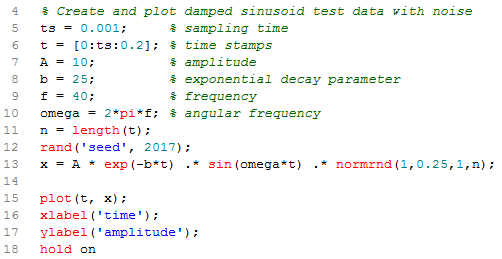
lsqcurvefitDemo.oml in
the<installation_dir>/tutorials/ folder folder. The
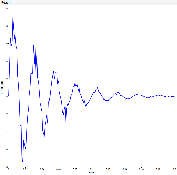
file contains code to create sampled data from a damped sinusoid response with
random noise.
The plot looks like this:
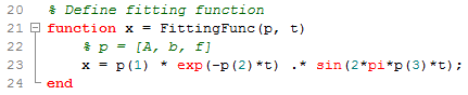
Define the Fitting Function
The parameters for the fitted curve are the amplitude, the exponential damping coefficient, and the oscillation frequency. The parameters are designated A, b and f, and they are passed to the fitting function in a vector as the first argument. The second argument is the vector of times at which the function is to be evaluated.
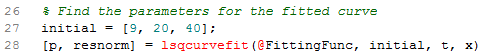
Perform the Curve Fit with lsqcurvefit
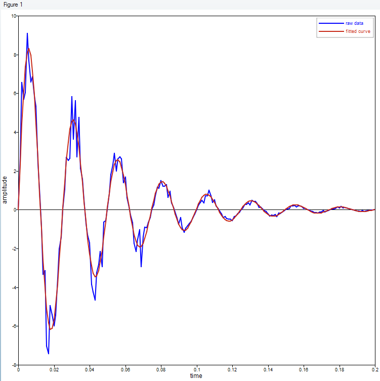
From the data plot and some calculations, we can estimate the fitting parameters. These initial estimates are required inputs for lsqcurvefit. The other inputs are the t and x raw data values.
The output is shown below:
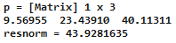
The first output, p, contains the fitted parameters. The second output, resnorm, contains the norm of the residual differences between the raw data and the fitted curve.
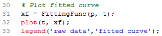
Plot the Fitted Curve with the Raw Data
Create Test Data for Fitting with polyfit
-
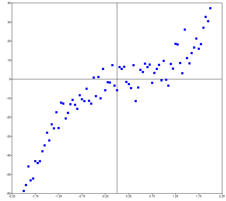
The file contains code to create data for a scatter plot with a polynomial
trend.
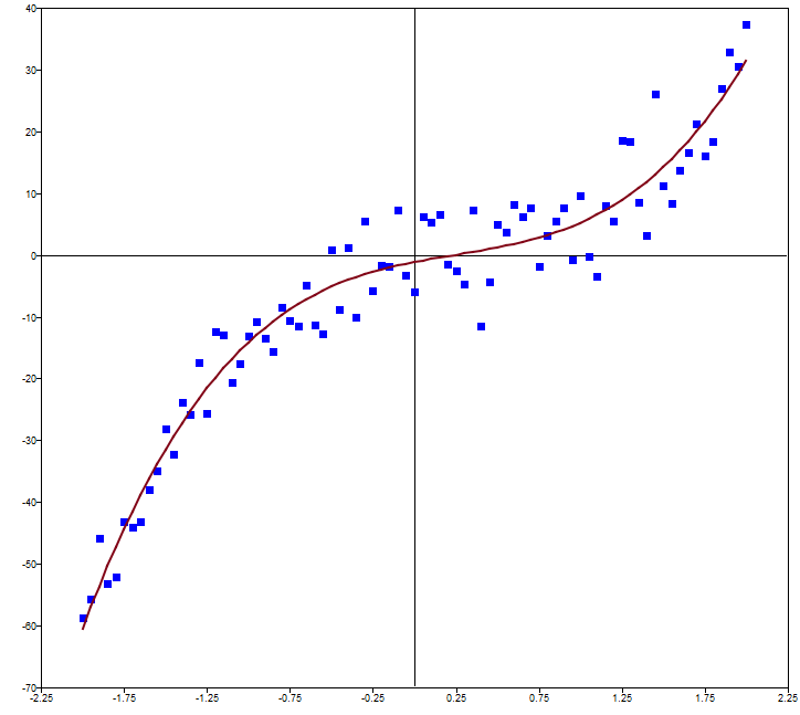
The plot looks like this:
Perform the Curve Fit with polyfit
From the data plot and some calculations, we can estimate the fitting parameters. These initial estimates are required inputs for polyfit. The other inputs are the t and x raw data values.

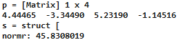
The output is shown below. The first output, p, contains the fitted polynomial coefficients. The second output, s, contains statistical data. Only the norm of the residuals vector is shown here.
Plot the Fitted Curve with the Raw Data
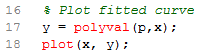
Using polyval with the coefficients (p) determined above, the fitted curve can be plotted together with the raw data.