Compose-4010: Solving Ordinary Differential Equations
This tutorial considers solving ordinary differential equations (ODE) in Compose OML language. A second order differential equation is used for illustration purposes as they are more common. The equation can represent a mechanical spring-mass-damper system or a series RLC circuit, both excited by an arbitrary sinusoidal input of amplitude A.

- Φ = the position
- α = the damping coefficient divided by the mass
- β = the spring stiffness divided by the mass
- The excitation is a force.
- Ф = the current
- α = the resistance divided by the inductance
- β = the reciprocal of the product of the capacitance and the inductance
- The excitation is a voltage whose derivative is A*sin(ωt).
Converting to First Order Equations
This is a required step since the ODE solvers can only solve first order explicit equations. This is done by introducing one additional state variable, ξ, to be equal to the derivative of the original state variable, Ф. There are two coupled first order differential equations:
The new state variable relationship equation:


Note that the equations are expressed in explicit form (only derivatives on the left side). The task is to solve these two coupled equations for the two-state variables as a function of time.
For the convenience of illustration, all of the parameters (α, β, A, ω) will be equal to 1.
Implementing the Two Equations
-
From the File menu, select Open and locate the file
ode45Demo.oml in the
<installation_dir>/tutorials/ folder.
This is what our system function looks like, using x in the code for the vector [φ, ξ].
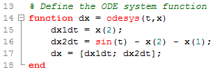
The system function implements the two equations derived above. The first argument is the current time, and the second argument contains the values of the state variables in a vector.
Using the ODE Solver

The first argument is for the ODE system function. The second argument is the vector of times at which to solve the equation. The third argument is the initial condition vector for the state variables. The default tolerances are explicitly specified in the options argument for illustration.
The time vector is reproduced as the first output argument. It is identical to the input for this case. The second output argument, x, contains the values of φ and ξ by column at each time in vector t.
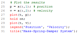
Plotting the Results
The following code extracts and plots the results.
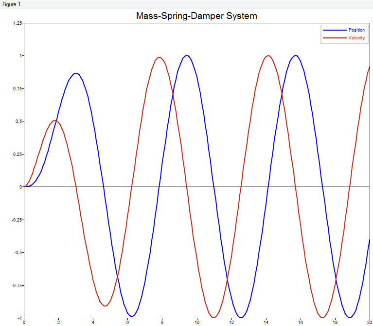
For a spring-mass-damper system, the plot represents the position and velocity. For the RLC circuit, the plot represents the current and its rate of change.