Stress-Life (S-N) Approach

S-N Curve

The S-N curve, first developed by Wöhler, defines a relationship between stress and number of cycles to failure. Typically, the S-N curve (and other fatigue properties) of a material is obtained from experiment; through fully reversed rotating bending tests. Due to the large amount of scatter that usually accompanies test results, statistical characterization of the data should also be provided (certainty of survival is used to modify the S-N curve according to the standard error of the curve and a higher reliability level requires a larger certainty of survival).

Figure 1. S-N Data from Testing

When S-N testing data is presented in a log-log plot of alternating nominal stress amplitude

S_{a}

$S_{a}$ or range

$S_{R}$ versus cycles to failure

$N$ , the relationship between

$S$ and

$N$ can be described by straight line segments. Normally, a one or two segment idealization is used.

Figure 2. One Segment S-N Curves in Log-Log Scale

(1)

$S = S 1 {(N_{f})}^{b 1}$

for segment 1

Where, $S$ is the nominal stress range, $N_{f}$ are the fatigue cycles to failure, $b_{l}$ is the first fatigue strength exponent, and $S I$ is the fatigue strength coefficient.

The S-N approach is based on elastic cyclic loading, inferring that the S-N curve should be confined, on the life axis, to numbers greater than 1000 cycles. This ensures that no significant plasticity is occurring. This is commonly referred to as high-cycle fatigue.

S-N curve data is provided for a given material .

Rainflow Cycle Counting

Cycle counting is used to extract discrete simple "equivalent" constant amplitude cycles from a random loading sequence. One way to understand "cycle counting" is as a changing stress-strain versus time signal. Cycle counting will count the number of stress-strain hysteresis loops and keep track of their range/mean or maximum/minimum values.

Rainflow cycle counting is the most widely used cycle counting method. It requires that the stress time history be rearranged so that it contains only the peaks and valleys and it starts either with the highest peak or the lowest valley (whichever is greater in absolute magnitude). Then, three consecutive stress points (1, 2, and 3) will define two consecutive ranges as

$Δ S_{12} = | S_{1} - S_{2} |$ and

$Δ S_{23} = | S_{2} - S_{3} |$ |. A cycle from 1 to 2 is only extracted if

$Δ S_{12} \leq Δ S_{23}$ . Once a cycle is extracted, the two points forming the cycle are discarded and the remaining points are connected to each other. This procedure is repeated until the remaining data points are exhausted.

Simple Load History:

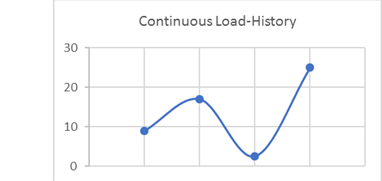
Figure 3. Continuous Load History

Since this load history is continuous, it is converted into a load history consisting of peaks and valleys only.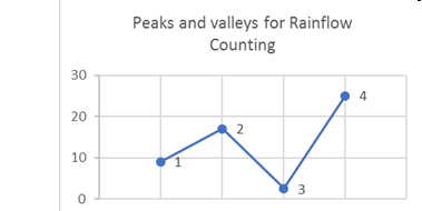

Figure 4. Peaks and Valleys for Rainflow Counting. 1, 2, 3, and 4 are the four peaks and valleys

It is clear that point 4 is the peak stress in the load history, and it will be moved to the front during rearrangement (Figure 5). After rearrangement, the peaks and valleys are renumbered for convenience.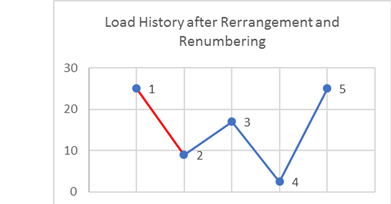

Figure 5. Load History after Rearrangement and Renumbering

Next, pick the first three stress values (1, 2, and 3) and determine if a cycle is present.

If $S_{i}$ represents the stress value, point $_{i}$ then:(2)
$Δ S_{12} = | S_{1} - S_{2} |$
(3)
$Δ S_{23} = | S_{2} - S_{3} |$

As you can see from Figure 5 , $Δ S_{12} \geq Δ S_{23}$ ; therefore, no cycle is extracted from point 1 to 2. Now consider the next three points (2, 3, and 4).(4)
$Δ S_{23} = | S_{2} - S_{3} |$
(5)
$Δ S_{34} = | S_{3} - S_{4} |$

$Δ S_{23} \leq Δ S_{34}$ , hence a cycle is extracted from point 2 to 3. Now that a cycle has been extracted, the two points are deleted from the graph.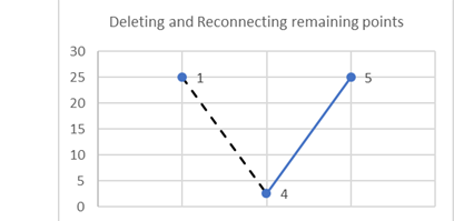

Figure 6. Delete and Reconnect Remaining Points

The same process is applied to the remaining points:(6)
$Δ S_{14} = | S_{1} - S_{4} |$
(7)
$Δ S_{45} = | S_{4} - S_{5} |$

In this case, $Δ S_{14} = Δ S_{45}$ , so another cycle is extracted from point 1 to 4. After these two points are also discarded, only point 5 remains; therefore, the rainflow counting process is completed.

Two cycles (2→3 and 1→4) have been extracted from this load history. One of the main reasons for choosing the highest peak/valley and rearranging the load history is to guarantee that the largest cycle is always extracted (in this case, it is 1→4). If you observe the load history prior to rearrangement, and conduct the same rainflow counting process on it, then clearly, the 1→4 cycle is not extracted.
Complex Load History
The rainflow counting process is the same regardless of the number of load history points. However, depending on the location of the highest peak/valley used for rearrangement, it may not be obvious how the rearrangement process is conducted. Figure 7 shows just the rearrangement process for a more complex load history. The subsequent rainflow counting is just an extrapolation of the process mentioned in the simple example above, and is not repeated here.

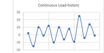
Figure 7. Continuous Load History

Since this load history is continuous, it is converted into a load history consisting of peaks and valleys only: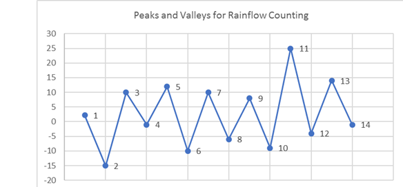

Figure 8. Peaks and Valleys for Rainflow Counting

Clearly, load point 11 is the highest valued load and therefore, the load history is now rearranged and renumbered.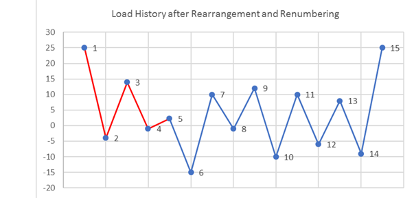

Figure 9. Load History After Rearrangement and Renumbering

The load history is rearranged such that all points including and after the highest load are moved to the beginning of the load history and are removed from the end of the load history.

Equivalent Nominal Stress

Since S-N theory deals with uniaxial stress, the stress components need to be resolved into one combined value for each calculation point, at each time step, and then used as equivalent nominal stress applied on the S-N curve.

Various stress combination types are available with the default being "Absolute maximum principle stress". "Absolute maximum principle stress" is recommended for brittle materials, while "Signed von Mises stress" is recommended for ductile material. The sign on the signed parameters is taken from the sign of the Maximum Absolute Principal value.

Mean Stress Correction

Generally, S-N curves are obtained from standard experiments with fully reversed cyclic loading. However, the real fatigue loading could not be fully-reversed, and the normal mean stresses have significant effect on fatigue performance of components. Tensile normal mean stresses are detrimental and compressive normal mean stresses are beneficial, in terms of fatigue strength. Mean stress correction is used to take into account the effect of non-zero mean stresses.

The Gerber parabola and the Goodman line in Haigh's coordinates are widely used when considering mean stress influence, and can be expressed as:

Gerber:(8)

$S_{e} = \frac{S_{r}}{(1 - {(\frac{S_{m}}{S_{u}})}^{2})}$

Goodman:(9)

$S_{e} = \frac{S_{r}}{(1 - \frac{S_{m}}{S_{u}})}$

Where,

$S_{m}$: Mean stress given by $S_{m} = (S_{m a x} + S_{m i n}) / 2$
$S_{r}$: Stress Range given by $S_{r} = S_{m a x} - S_{m i n}$
$S_{e}$: Stress range after mean stress correction (for a stress range $S_{r}$ and a mean stress $S_{m}$ )
$S_{u}$: Ultimate strength

The Gerber method treats positive and negative mean stress correction in the same way that mean stress always accelerates fatigue failure, while the Goodman method ignores the negative means stress. Both methods give conservative result for compressive means stress. The Goodman method is recommended for brittle material while the Gerber method is recommended for ductile material. For the Goodman method, if the tensile means stress is greater than UTS, the damage will be greater than 1.0. For the Gerber method, if the mean stress is greater than UTS, the damage will be greater than 1.0, with either tensile or compressive.

A Haigh diagram characterizes different combinations of stress amplitude and mean stress for a given number of cycles to failure.

Figure 10. Haigh Diagram and Mean Stress Correction Methods

Parameters affecting mean stress influence

FKM:

Regime 1 (R > 1.0): $S_{e}^{A} = S_{a} (1 - M)$
Regime 2 (-∞ ≤ R ≤ 0.0): $S_{e}^{A} = S_{a} + M * S_{m}$
Regime 3 (0.0 < R < 0.5): $S_{e}^{A} = (1 + M) \frac{S_{a} + (\frac{M}{3}) S_{m}}{1 + \frac{M}{3}}$
Regime 4 (R ≥ 0.5): $S_{e}^{A} = \frac{3 S_{a} {(1 + M)}^{2}}{3 + M}$

Where,

$S_{e}^{A}$: Stress amplitude after mean stress correction (Endurance stress)
$S_{m}$: Mean stress
$S_{a}$: Stress amplitude

If all four are specified for mean stress correction, the corresponding Mean Stress Sensitivity values are slopes for controlling all four regimes. Based on FKM-Guidelines, the Haigh diagram is divided into four regimes based on the Stress ratio ( $R = S_{\min} / S_{\max}$ ) values. The Corrected value is then used to choose the S-N curve for the damage and life calculation stage.

Regime 1 (R > 1.0)
Regime 2 (-∞ ≤ R ≤ 0.0)
Regime 3 (0.0 < R < 0.5)
Regime 4 (R ≥ 0.5)

Where,

$S_{m}$: Mean stress
$S_{a}$: Stress amplitude
$M_{i}$

Damage Accumulation Model

Palmgren-Miner's linear damage summation rule is used. Failure is predicted when:(10)

$\sum D_{i} = \sum \frac{n_{i}}{N_{i f}} \geq 1.0$

Where,

$N_{i f}$: Materials fatigue life (number of cycles to failure) from its S-N curve at a combination of stress amplitude and means stress level $i$ .
$n_{i}$: Number of stress cycles at load level $i$ .
$D_{i}$: Cumulative damage under $n_{i}$ load cycle.

The linear damage summation rule does not take into account the effect of the load sequence on the accumulation of damage, due to cyclic fatigue loading. However, it has been proved to work well for many applications.