Contour Plots

The Contour panel allows you to contour a model and graphically visualize the results. In the Contour panel you can view vector, tensor, or scalar type results. To access the Contour panel either click the Contour panel icon on the Results toolbar, or select Results > Plot > Contour from the menu bar.

Averaging Method

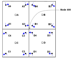
Nodal averaging of elemental results is available in HyperView. Nodal averaging of elemental results at a node refers to the average of all the element corner results passing through that node. If no corner results are available for an element, centroidal results will be used to calculate the nodal average. In the example to the right, four elements are passing through Node 400. The average results at Node 400 is equal to:.

Variation (%)

The Variation (%) is the relative difference at a node with respect to all nodes in the selected components. The formula is described as follows:

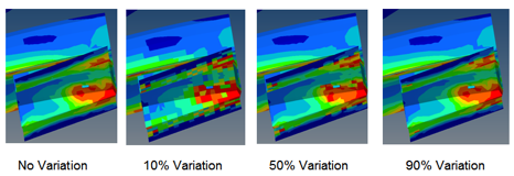
You can activate Variation (%) in the Contour panel and select a specific variation percentage to control the nodal averaging calculation.

If Variation (%) is off, the average results are calculated for all nodes. In this case, the results are node bound, meaning you can query results at a node from the Query panel.

If Variation (%) is on, the average results are calculated for only some nodes, depending on the variation (%) you have defined.

If the variation percentage is below the designated value at a node, nodal average at that node is calculated. Otherwise, corresponding element corner results at that node are used for contour plotting.

100% Variation indicates all nodes will have average results; 0% Variation indicates no nodes will have average results. In this case, the results are element bound, meaning you can only query results at an element from the Query panel.

Contour Plots using the Results Browser

Within the Results Browser there is the Result View. The Result View shows a hierarchical view of available results for the current load case. The result types are grouped by their type, and are broken up into Scalar, Vector, and Tensor folders. You can expand the folder to see all of the details for each result type. For example, each of the Scalar, Tensor, and Vector folders are expanded to see the Result Type within the folders. By selecting one of those Result Types (for instance, Displacement Magnitude), the different Components are shown:

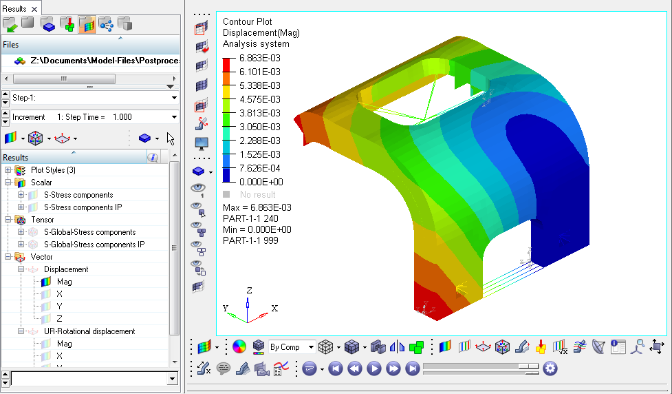
To apply a contour plot using the Results Browser, simply click on the icon to the left of the result to be used for the contour. For example, in the image below, the Displacement component is contoured. Click Mag, X, Y, or Z to change the contour in the image.

The Layer selector allows you to quickly go through the various layers of the current result plots (contour, tensor, or vector). This selector is located at the bottom of the browser, and is available in the Result View only.

The Layer selector list is refreshed whenever a data type or the component of the data type is selected in the tree.

You can change the current layer by clicking the up/down arrows on the Layer selector, or by using the drop-down menu to select a layer from the layer list. A contour plot of the selected result and layer will automatically be applied whenever the layer is changed. In the example below, the component vonMises Stress contoured. You can change the layer by selecting the layer as shown in the drop down menu.

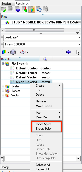
Also within the Results Browser is a folder named Plot Styles. Plot Styles are a collection of predefined settings for a contour, vector, or tensor plot. For example, using the Contour panel, various aspects of a contour such as averaging method, display options, and result type are set.

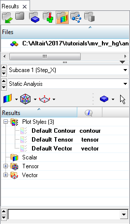
To create a Plot Style, the Contour panel is used to create a contour plot. Once the contour is displayed in the Graphics Area, the Create Plot Styles… button can be selected:

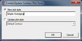
This allows you to save settings that you use often. For example, above the plot style Simple Averaging was created. We can also create another plot style called My Defaults that specifies that no averaging should be done. Using the Result View in the Results Browser, the Current Plot Style can be set either using the Quick Plot toolbar (shown below) or by right clicking on the plot style and selecting Make Current.

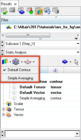
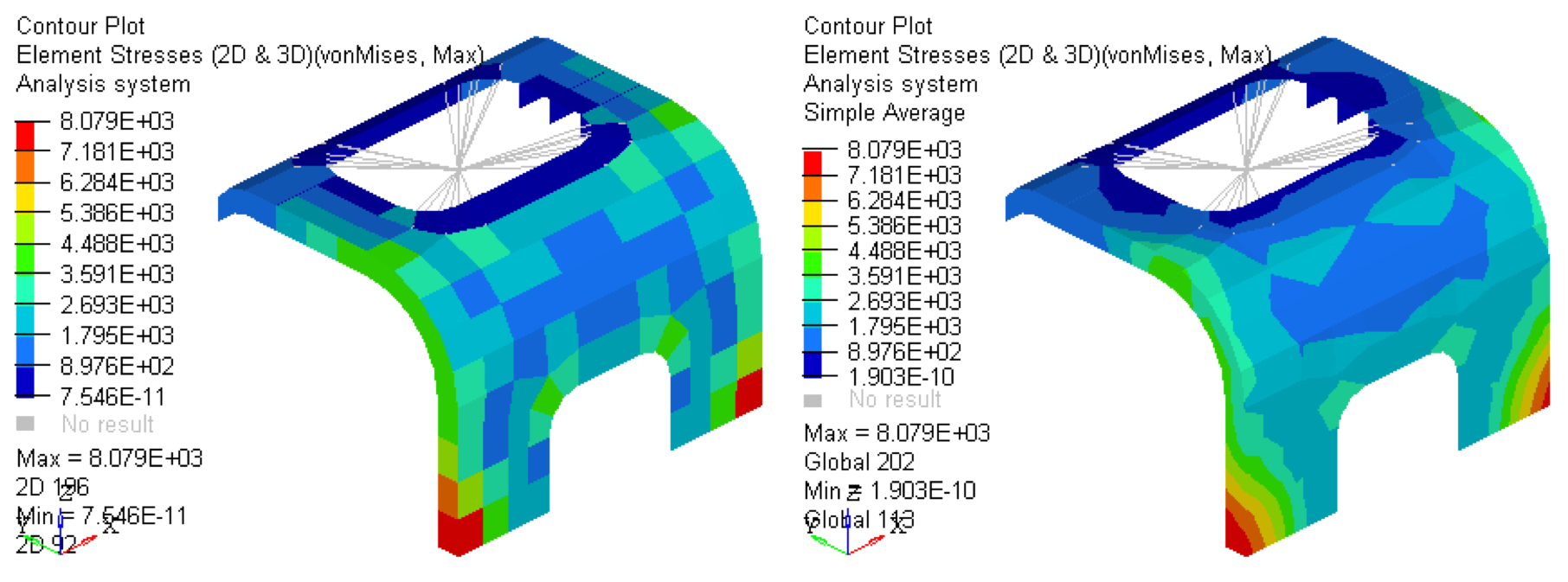
Once a contour plot style is selected as Current, the settings in that plot style will be used when a result type is selected for contouring. For example, the image to the left uses the Default Contour plot style that is loaded into each HyperWorks Desktop Session, while the image to the right uses the Simple Averaging plot style that we previously created.

The predefined plot styles come initially from a file in your HyperWorks installation directory. You can export your own plot styles and make them your default by bringing up the browser context menu in the Result Browser and clicking Export Styles. The styles will be written out in XML format to a file you define. You can use these styles as your own default by changing the DefaultPlotStyles line in your preference file. Simply set the path and file name to your plot styles file. You can also import plot styles using the Import Styles option in the browser context menu (or the Tools menu).