What's New
View new features for MotionSolve 2020.1.
General
New Features
- Support OML-based Subroutines
- MotionSolve supports subroutines that are scripted in the OpenMatrix Language (OML) using an embedded OML interpreter. The basic OML interpreter supports the basic OML syntax, but does not include/support any of the additional toolboxes and libraries. OML-based subroutines are supported on Windows only. A Linux support for OML subroutines will be provided in future releases. Furthermore, MotionSolve looks for a MATLAB installation to interpret *.m files. If the respective interpreter is not installed, MotionSolve uses its own basic OML interpreter to run *.m scripts instead.
- PSTATE for Linear Analysis
- You can define your own states via a new PSTATE modeling element. Each PSTATE contains a list of VARIABLES that have been defined in the model. These VARIABLES define the states to use in the linearization. MotionSolve uses these states for generating the linear problem. PSTATE is currently supported in MotionSolve through .xml input files or the MSolve API only. MotionView will support this feature in a future release. For more information on PSTATE, please see the Reference: PlantState command in the MotionSolve Reference Guide.
Enhancements
- Descriptor State Space
- MotionSolve is able to generate matrices for state-space representation during a linear analysis step. The respective matrices (A, B, C, D) describe a mathematical model of a physical system as a set of input, output, and state variables related by first-order differential equations. Until now, MotionSolve only supported forces as inputs for state-space generation. In this release, you can define motion as inputs as well, which will result in a linear implicit model. The motions are added as algebraic constraints which leads to a descriptor state-space representation on the form of Eẋ = Ax + Bu and y = Cx + Du, where x is the state vector, u is the input vector, and y is the output vector. Descriptor State Space is currently supported in MotionSolve through .xml input files or the Msolve API; it is not available through MotionView. For more information on PSTATE, please see the Parameters: Linear Solver command in the in the MotionSolve Reference Guide.
Resolved Issues
- The Linux installer returned an error message regarding the lack of disc space for the root directory, even if you want to install the solver within another directory or drive.
- In some cases, an inside cylinder got “shot away” within a cylinder-inside-cylinder contact if the penetration between the inside and outside cylinder was excessive.
- Some Functional Mock-up Units based on Model Exchange were not solved correctly in MotionSolve.
- After a Save and Load command, the internal states corresponding to the Motion Marker B1/B2/B3 were not initialized correctly, causing an offset between Motion states and the corresponding AX/AY/AZ values saved to the XML file. This caused some discontinuities in the results after the reload.
- MotionSolve FMU generated by MotionView were not running in Activate on Linux.
- MotionSolve Subroutine Builder failed to execute on the Linux platform.
Altair MotionSolve 2020 Release Notes
Linear Analysis
New Features
- A, B, C, and D State Matrices in OML Format
- MotionSolve can create state space matrices in the OpenMatrix Language (OML) format. You can directly load these matrices into Compose and Activate for further analysis.
- Kinetic and Strain Energy for Flexible Bodies
- MotionSolve can calculate the kinetic/strain energies and dissipative power for flexible bodies that are defined using Component Mode Synthesis (CMS).
- Modal Energy Distribution
- MotionSolve can write an HTML file with the modal energy distributions. The HTML file aids in understanding how the energies are distributed across the different mode shapes.
Enhancements
- PINSUB and POUTSUB
- PINSUB and POUTSUB are available as Python sub-routines.
Known Issues
- Linear Analysis reports 0Hz for frequency dependent bushings.
- Linear Analysis fails with NLFE bodies.
- Linear Analysis fails if the mass of a body is 0.
- GCON and PFORCE are not supported for Linear Analysis.
- Only 1 linear analysis at a time can be performed.
- Linear analysis needs to be the last simulation step in a sequence.
Resolved Issues
- Eigenmodes were not displayed correctly in HyperView for some models.
- Linear Analysis with tire models sometimes caused a software crash.
Rigid Body Contact
Enhancements
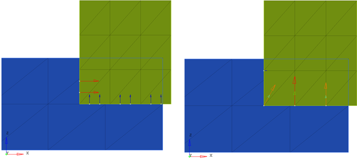
- 3D Meshed Contact
- The 3D meshed contact algorithm has been enhanced
with an additional optional node-based method for computing the
contact kinematics. This feature calculates the normal forces on the
nodes of the surface mesh, instead of the center of the mesh
triangles. The node-centric contact feature provides improved
accuracy, particularly in situations where large penetration occurs
due to sharp edges in contact.Figure 1. Extreme contact penetration example. (Left) Contact Forces acting on element center. (Right) New node-based contact feature with reaction forces acting on nodes. Note that at the edge on the lower left of the green box, the contact force is inclined as expected.
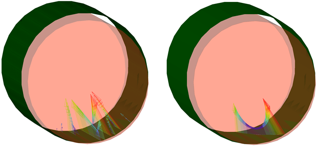
- Cylinder in Cylinder Contact
- The contact model in MotionSolve allows the contact between a cylinder
inside another cylinder to be calculated analytically using the
is_material_inside flag. Also, cylinder inside
cylinder is supported for open and capped cylinders (inside and
outside). The analytical contact formulation has advantages in terms of
speed and accuracy compared to the mesh-based contact calculation.Figure 2. Cylinder in cylinder contact. (Left) Mesh-based contact calculation. (Right) Analytical-based contact analysis. Note that the contact force distribution is much smoother for analytical contact.
Known Issues
- The node-centric feature of the 3D meshed contact can provide inaccurate results for complicated-shaped contact patches. In these situations, you are encouraged to simulate contact with reaction forces resolved at the element center.
Resolved Issues
- Cylinder caps improvement implemented, where top and bottom caps had been mixed up.
Co-Simulation with EDEM
New Features
- Linux Support
- In the 2019.1 release, MotionSolve added a new feature to co-simulate with the bulk material simulation software EDEM. This release expands support of the MotionSolve/EDEM co-simulation for the Linux operating system.
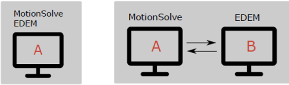
- Cross-platform Support
- You can run a MotionSolve and EDEM co-simulation on two separate
machines via a network connection. The simulation can be of heterogenous
operating systems, meaning MotionSolve can run on Windows while EDEM
runs on the Linux operating system and vice versa.Figure 3. (Left) Co-simulation on the same machine. (Right) Simulation of cross-platform.
- Batch Simulation
- A batch script allows you to provide multiple input files and run multiple simulations with these inputs in sequence.
Enhancements
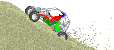
- H3D File Generation
- H3D generation of EDEM particles is now optional, which improves memory
usage and performance during large simulations. Furthermore, the EDEM
H3D file has been redesigned and can be loaded faster into
HyperView.Figure 4. Visualizing MotionSolve and EDEM results within HyperView.
- Coupling at T > T0
- MS/EDEM co-simulation supports starting a coupled simulation at T > T0, meaning that MotionSolve simulates the system without EDEM running from T0 (start time) to T (coupling time), at which point co-simulation starts.
Known Issues
- Simulation using the batch script ends with an error message and no H3D file is generated for the EDEM particles. However, EDEM still creates an H5 result file. You can manually convert the H5 file into H3D using edem2h3d.py script.
Resolved Issues
- A memory leak in the H3D generation.
Co-Simulation with FMU
New Features
- Coupling at T > T0
- The co-simulation capabilities of MotionSolve with Functional Mockup Units (FMU) allows starting a coupled simulation at T > T0, meaning MotionSolve simulates the system without the FMU from T0 (start time) to T (coupling time). This allows for computational performance improvements where the dynamic influence of the FMU is only relevant at time greater than T0, and where the FMU is computationally expensive (example: FE based model).
- Kinematic Analysis
- The co-simulation capabilities of MotionSolve with FMU supports kinematic analysis.
Enhancements
- Additional Debugging Capabilities
- You can increase the solver log related specifically to FMUs. This can
be done by setting the environment variable MS_FMU_LOGGING_LEVEL=…
- ALL – Log all messages.
- WARNING – Log messages every time the FMU returns a warning status for any of its functions.
- ERROR - Log messages every time the FMU returns an error status for any of its functions.
- FATAL - Log messages every time the FMU returns a fatal error status for any of its functions.
- Compliance Checks
- Improved compliance checks make the co-simulation with FMUs more robust. Here, the validity of the FMU is being checked against the FMI standard and warnings/errors are being reported in situations where the FMU does not comply with the standard.
Resolved Issues
- The FMU temp folder was not deleted after a completed simulation.
User Subroutines
New Features
- New XML Configuration File
- A new XML configuration file allows you to customize the UserSubBuildTool.exe for your environment.
Enhancements
- Visual Studio and Fortran
- User subroutines support Visual Studio 2005–2019 and Intel Fortran 10–2020. Furthermore, the installation of a Fortran compiler is no longer necessary if the subroutine consists of C/CPP files only. In such cases, you only require Visual Studio (the Fortran compiler is not needed).
Miscellaneous
Enhancements
- Active State Python
- The Python implementation in MotionSolve is now based on Active State Python 3.5.4.
Resolved Issues
- After a reload, results of a model with COUXX2 were discontinuous.
- The damping ratios generated by MotionView were not scaled properly if non-default units were used during a CMS run in OptiStruct.
- The distributed load on a flexible body has two components: a rigid body component that has a tendency to accelerate the flexible body that it is acting on, and, a modal component that has a tendency to deform the flexible body that it is acting on. The distributed force created by Force_FlexModal was not scaled correctly on the rigid body component when non-default units were used.