RD-V: 0505 Shock Tube

The transitory response of a perfect gas in a long tube separated into two parts using a diaphragm is studied. The problem is well-known as the Riemann problem. The numerical results based on the finite element method with the Lagrangian and Eulerian formulations, are compared to the analytical solution.

This famous experiment is interesting for observing the shock-wave propagation. Moreover, this case uses the representation of perfect gas and compares the different formulations: The ALE uses Lagrangian or Eulerian.

The first part of the study deals with the modeling description of perfect gas with the hydrodynamic viscous fluid LAW6. The purpose is to test the different formulations:

Lagrangian (mesh points coincident to material points)
Eulerian (mesh points fixed)

The propagation of the gas in the tube can be studied in an analytical manner. The gas is separated into different parts characterizing the expansion wave, the shock front and the contact surface. The simulation results are compared with the analytical solution for velocity, density and pressure.

Options and Keywords Used

Brick elements
Lagrangian and Eulerian formulations
Hydrodynamic viscous fluid law (/MAT/LAW6 (HYDRO or HYD_VISC)) and perfect gas modeling
ALE boundary conditions (/ALE/BCS)
ALE material formulation (/ALE/MAT)

Input Files

The input files used in this example include:

<install_directory>/hwsolvers/demos/radioss/verification/Blast/0505_shock_tube/*

Model Description

The shock tube problem is one of the standard problems in gas dynamics. It is a very interesting test since the exact solution is known and can be compared with the simulation results. The Finite Element method using the Eulerian and Lagrangian formulations was used in the numerical models.

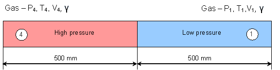
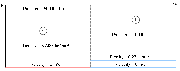
A shock tube consists of a long tube filled with the same gas in two different physical states. The tube is divided into two parts, separated by a diaphragm. The initial state is defined by the values for density, pressure and velocity, as shown in Figure 2 and Figure 3. All the viscous effects are negligible along the tube sides; it is also assumed that there is no motion in the beginning.

The initial state at time t = 0 consists of two constant states 1 and 4 with $p_{4} > p_{1}$ , $ρ_{4} > ρ_{1}$ , and $v_{4} = v_{1} = 0$ (table).

Table 1. Initial Conditions in the Shock Tube
	High pressure side (4)	Low pressure side (1)
Pressure $p$	500000 $[Pa]$	20000 $[Pa]$
Velocity $v$	0 $[\frac{m}{s}]$	0 $[\frac{m}{s}]$
Density $ρ$	5.7487 $[\frac{k g}{m m^{3}}]$	0.22995 $[\frac{k g}{m m^{3}}]$
Temperature $T$	303 $[K]$	303 $[K]$

Just after the membrane is removed, a compression shock runs into the low pressure region, while a rarefaction (decompression) wave moves into the high pressure part of the tube. Furthermore, a contact discontinuity usually occurs.

Model Method

The hydrodynamic viscous fluid LAW6 is used to describe compressed gas.

The general equation describing pressure is:(1)

$p = C_{0} + C_{1} μ + C_{2} μ^{2} + C_{3} μ^{3} + (C_{4} + C_{5} μ) E$

With $μ = \frac{ρ}{ρ_{0}} - 1$

Where,

$p$: Pressure
$C_{i}$: Hydrodynamic constants
$E_{n}$: Internal energy per initial volume
$ρ$: Density

Perfect gas is modeled by setting all coefficients:(2)

$C_{0} = C_{1} = C_{2} = C_{3} = 0$ And

$C_{4} = C_{5} = γ - 1$

Where, $γ$ is the gas constant.

Then the initial internal energy, per initial volume is calculated from initial pressure:(3)

$E_{0} = \frac{p_{0}}{γ - 1}$

Under the assumption $γ = c o n s t . = 1.4$ (valid for low temperature range), the hydrodynamic constants $C_{4} = C_{5} = 0.4$ .

Gas pressure is described by:(4)

$p = (C_{4} + C_{5} μ) E$

(5)

$p = (0.4 + 0.4 \frac{ρ - ρ_{0}}{ρ_{0}}) E$

(6)

$E_{0} = \frac{p_{0}}{0.4}$

Parameters of material LAW6 are provided in Table 2.

Table 2. Material Properties of Gas in LAW6
	High Pressure Side (4)	Low Pressure Side (1)
Initial volumetric energy density (`E`₀)	1.25x10⁶ $[\frac{J}{m m^{3}}]$	5x10⁴ $[\frac{J}{m m^{3}}]$
$C_{4}$ and $C_{5}$	0.4	0.4
Density $ρ$	5.7487 $[\frac{k g}{m m^{3}}]$	0.22995 $[\frac{k g}{m m^{3}}]$

Analytical Approach

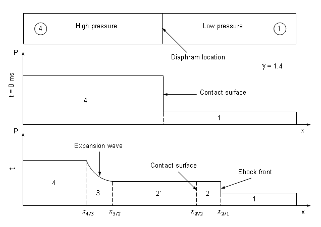
The shock tube problem has an analytical solution of time before the shock hits the extremity of the tube. ¹

Evolution of the flow pattern is illustrated in Figure 4. When the diaphragm bursts, discontinuity between the two initial states breaks into leftward and rightward moving waves, separated by a contact surface.

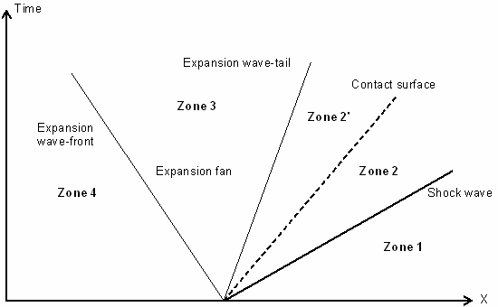
Each wave pattern is composed of a contact discontinuity in the middle and a shock or a rarefaction wave on the left and the right sides separating the uniform state solution. The shock wave moves at a supersonic speed into the low pressure side. A one-dimensional problem is considered.

There are four distinct zones marked 1, 2, 3 and 4 in Figure 5.

Zone 1 is the low pressure gas which is not disturbed by the shock wave.
Zone 2 (divided in 2 and 2' by the contact surface) contains the gas immediately behind the shock traveling at a constant speed. The contact surface across which the density and the temperature are discontinuous lies within this zone.
The zone between the head and the tail of the expansion fan is noted as Zone 3. In this zone, the flow properties gradually change since the expansion process is isentropic.
Zone 4 denotes the undisturbed high pressure gas.

Equations in Zone 2 are obtained using the normal shock relations. Pressure and the velocity are constant in Zones 2 and 2'.

The ratio of the specific heat constant of gas $γ$ is fixed at 1.4. It is assumed that the value does not change under the temperature effect, which is valid for the low temperature range.

The analytical solution to the Riemann problem is indicated at t=0.4 ms. A solution is given according to the distinct zones and continuity must be checked. Evolution in Zones 2 and 3 is dependent on the constant conditions of Zone 1 and 4. The analytical equations use pressure, velocity, density, temperature, speed of sound through gas and a specific gas constant. Equations in Zone 2 are obtained using normal shock relations and the gas velocity in Zone 2 is constant throughout. The shock wave and the surface contact speeds make it possible to define the position of the zone limits.

Zone 1:
Pressure $p$: $p_{1}$ = 20000 $[Pa]$
Velocity $v$: $v_{1} = 0$ $[\frac{m}{s}]$
Density $ρ$: $ρ_{1}$ = 0.22995 $[\frac{k g}{m m^{3}}]$
Temperature $T$: $T_{1}$ = 303 $[K]$

Zone 4:
Pressure $p$: $p_{4}$ = 500000 $[Pa]$
Velocity $v$: $v_{4} = 0$ $[\frac{m}{s}]$
Density $ρ$: $ρ_{4}$ = 5.7487 $[\frac{k g}{m m^{3}}]$
Temperature $T$: $T_{4}$ = 303 $[K]$

Speed of sound through gas:(7)

$a = \sqrt{\frac{p \cdot γ}{ρ}}$

Specific gas constant:(8)

$R = \frac{a^{2}}{T \cdot γ}$

Low Pressure Side (1):
$a_{1}$: = 348.95 $[\frac{m}{s}]$
R: 287.049 $[\frac{J}{kg \cdot K}]$

High Pressure Side (4):
$a_{4}$: = 348.95 $[\frac{m}{s}]$
R: 287.049 $[\frac{J}{kg \cdot K}]$

Zone 2:: Analytical Solution
Pressure $p$: $\frac{p_{4}}{p_{1}} = \frac{p_{2}}{p_{1}} {(1 - \frac{(γ - 1) \cdot (\frac{a_{2}}{a_{1}}) \cdot (\frac{p_{2}}{p_{1}} - 1)}{\sqrt{2 γ [2 γ + (γ + 1) \cdot (\frac{p_{2}}{p_{1}} - 1)]}})}^{\frac{- 2 γ}{γ - 1}}$
Velocity $v$: $v_{2} = \frac{a_{1}}{γ} (\frac{p_{2}}{p_{1}} - 1) {(\frac{\frac{2 γ}{(γ + 1)}}{\frac{p_{2}}{p_{1}} + (γ - 1) / (γ + 1)})}^{\frac{1}{2}}$
Density $ρ$: $ρ_{2} = ρ_{2} R T_{2}$
Temperature $T$: $\frac{T_{1}}{T_{2}} = \frac{p_{2}}{p_{1}} (\frac{\frac{(γ + 1)}{(γ - 1)} + \frac{p_{2}}{p_{1}}}{1 + (\frac{p_{2}}{p_{1}}) \cdot (\frac{(γ + 1)}{(γ - 1)})})$

Zone 2:: Results at t = 0.4 ms
Pressure $p$: $p_{2}$ = 80941.1 $[Pa]$
Velocity $v$: $v_{2} = 399.628$ $[\frac{m}{s}]$
Density $ρ$: $ρ_{2}$ = 0.5786 $[\frac{k g}{m m^{3}}]$
Temperature $T$: $T_{2} = 487.308$ $[K]$

Shock wave speed:(9)

$v_{s} = a_{1} \sqrt{\frac{γ + 1}{2 γ} (\frac{p_{2}}{p_{1}} - 1) + 1} = 663.166$

$[\frac{m}{s}]$

Therefore,

$x_{\frac{2}{1}} = 0.4 v_{s} + 500 = 765.266 [mm]$

Zone 2':: Analytical Solution
Pressure $p$: $p_{2} = p_{2}'$
Velocity $v$: $v_{2} = v_{2'}$
Density $ρ$: $ρ_{2'} = ρ_{3} (x_{4 / 3})$
Temperature $T$: $ρ_{2'} = r_{2'} R T_{2'}$

Zone 2':: Results at t = 0.4 ms
Pressure $p$: $p_{2}' = 80941.1$ $[Pa]$
Velocity $v$: $v_{2'} = 399.628$ $[\frac{m}{s}]$
Density $ρ$: $ρ_{2'} = 1.5657$ $[\frac{k g}{m m^{3}}]$
Temperature $T$: $T_{2'} = 180.096$ $[K]$

Surface contact speed: $v_{c} - v_{2}$

Therefore, $x_{\frac{2}{2'}} = 0.4 v_{s} + 500 = 659.85 [mm]$

Zone 3

Zone 3 is defined as:(10)

$- a_{4} \leq \frac{X}{t} \leq v_{3} - a_{3}$

Where, $x = X + 500$

At $v_{3} - a_{3} = - a_{4} = - 348.95$ $[\frac{m}{s}]$ $\Rightarrow X = - 348.95 t$

$\Rightarrow x_{\frac{4}{3}} (t = 0.4) = 360.42$ $[mm]$

At $v_{3} - a_{3} = v_{2} - a_{2'} = v_{2} - \sqrt{\frac{p_{2} γ}{p_{2'}}} = 130.602$ $[\frac{m}{s}]$ $\Rightarrow - 348.95 t \leq X \leq 130.602 t$

$\Rightarrow x_{\frac{3}{2'}} (t = 0.4) = 552.24$

$[mm]$

Zone 3:: Analytical Solution
Pressure $p$: $\frac{p_{3}}{p_{4}} = {(1 - \frac{(γ - 1)}{2} \frac{v_{3}}{a_{4}})}^{\frac{2 γ}{γ - 1}}$
Velocity $v$: $v_{3} = \frac{2}{γ + 1} (a_{4} + \frac{X}{t})$
Density $ρ$: $\frac{ρ_{3}}{ρ_{4}} = {(\frac{p_{3}}{p_{4}})}^{- γ}$
Temperature $T$: $\frac{p_{3}}{p_{4}} = {(\frac{T_{3}}{T_{4}})}^{\frac{γ}{γ - 1}}$

Zone 3:: Results at t = 0.4 ms
Pressure $p$: $p_{3} = 500000 {(1 - 0.2 (\frac{v_{3} (X)}{348.95}))}^{7}$
Velocity $v$: $v_{3} = 290.792 + 2.0833 X$
Density $ρ$: $ρ_{3} = 5.7487 {(\frac{p_{3} (X)}{500000})}^{\frac{1}{1.4}}$
Temperature $T$: $T_{3} = 303 {(\frac{p_{3} (X)}{500000})}^{\frac{1}{3.5}}$

Continuity verifications:(11)

$v_{3} (X_{\frac{3}{2'}}) = v_{2'} (X_{\frac{3}{2'}})$

(12)

$v_{3} (X_{\frac{4}{3}}) = v_{4} (X_{\frac{4}{3}})$

(13)

$p_{3} (X_{\frac{3}{2'}}) = p_{2'} (X_{\frac{3}{2'}})$

(14)

$p_{3} (X_{\frac{4}{3}}) = p_{4} (X_{\frac{4}{3}})$

(15)

$ρ_{3} (X_{\frac{3}{2'}}) = ρ_{2'} (X_{\frac{3}{2'}})$

(16)

$ρ_{3} (X_{\frac{4}{3}}) = ρ_{4} (X_{\frac{4}{3}})$

(17)

$T_{3} (X_{\frac{3}{2'}}) = T_{2'} (X_{\frac{3}{2'}})$

(18)

$T_{3} (X_{\frac{4}{3}}) = T_{4} (X_{\frac{4}{3}})$

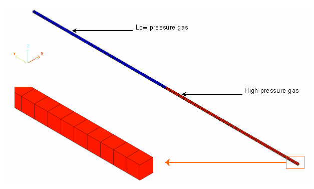
Finite Element Modeling with Lagrangian and Eulerian Formulations

Gas is modeled by 200 ALE bricks with solid property TYPE14 (general solid).

The model consists of regular mesh and elements, the size of which is 5 mm x 5 mm x 5 mm.

In the Lagrangian formulation, the mesh points remain coincident with the material points and the elements deform with the material. Since element accuracy and time step degrade with element distortion, the quality of the results decreases in large deformations.

In the Eulerian formulation, the coordinates of the element nodes are fixed. The nodes remain coincident with special points. Since elements are not changed by the deformation material, no degradation in accuracy occurs in large deformations.

The Lagrangian approach provides more accurate results than the Eulerian approach, due to taking into account the solved equations number.

For the ALE boundary conditions (/ALE/BCS), constraints are applied on:

Material velocity
Grid velocity

The nodes on extremities have material velocities fixed in X and Z directions. The other nodes have material and velocities fixed in X, Y and Z directions.

The ALE materials have to be declared Eulerian or Lagrangian with /ALE/MAT.

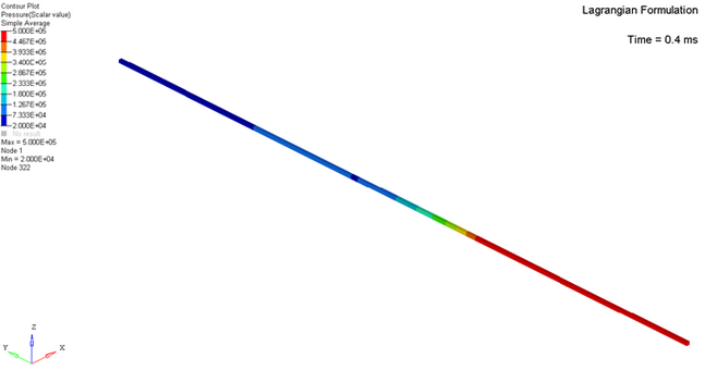
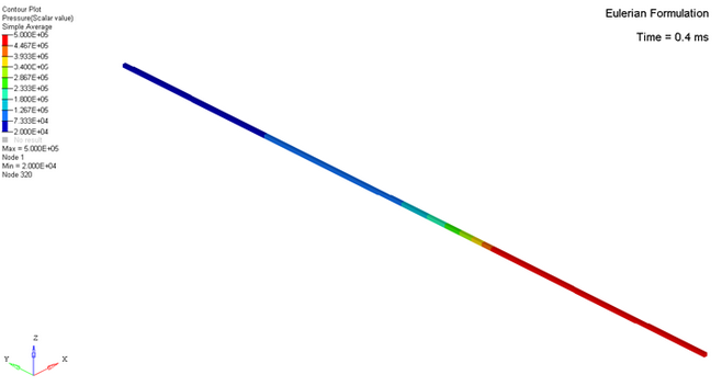
Results

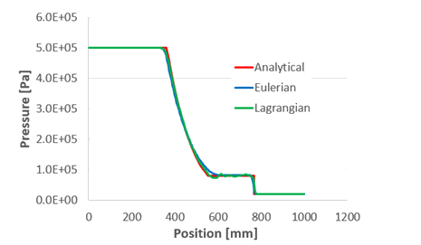
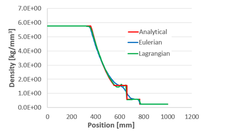
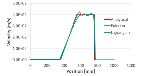
Finite Element Results and Analytical Solution Comparison

Simulation results along the tube axis at 0.4 ms are shown in the following diagrams.

Lagrangian Formulation
Scale factor: $Δ t_{s c a} = 0.1$

Eulerian Formulation
Scale factor: $Δ t_{s c a} = 0.5$

Pressure Distribution

Pressure wave produced in the shock-tube at t = 0.4 ms

J. D. Anderson Jr., Modern Compressible Flow with Historical Perspective, McGraw Hill Professional Publishing, 2nd ed., Oct. 1989