Spring Hardening

Isotropic, kinematic or uncoupled spring hardening options can be defined by the hardening flag $H$ .

These examples only include the spring stiffness without any damping.

Linear Elastic Spring, H=0

A linear spring can be modeled by inputting only the linear stiffness as

$K_{i}$ and fct_ID_1i =fct_ID_4i =0. For linear spring,

$H$ is always 0.

Figure 1. Linear Elastic Spring. with

$H$ =0

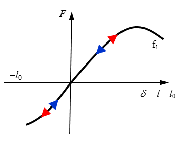
Nonlinear Elastic Spring, H=0

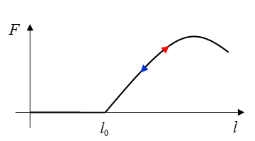
A nonlinear elastic spring is modeled by defining a force versus displacement curve where

$f_{1}$ in Figure 2 is defined in fct_ID_1i. Since the model is elastic, the loading and unloading follow the same path.

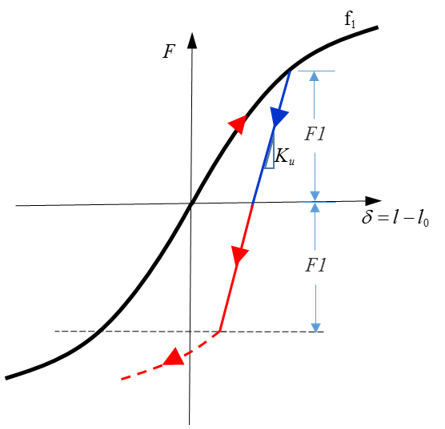
Nonlinear Elastic Plastic Spring with Isotropic Hardening, H=1

Figure 3 shows the behavior of a nonlinear elastic plastic spring with isotropic hardening where

$f_{1}$ is defined in fct_ID_1i and unloading stiffness

$K_{u}$ is input using

$K_{i}$ .

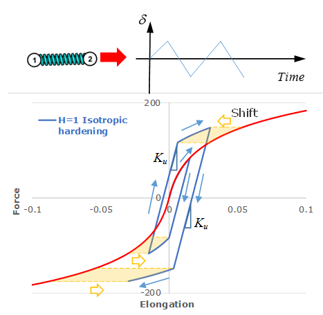
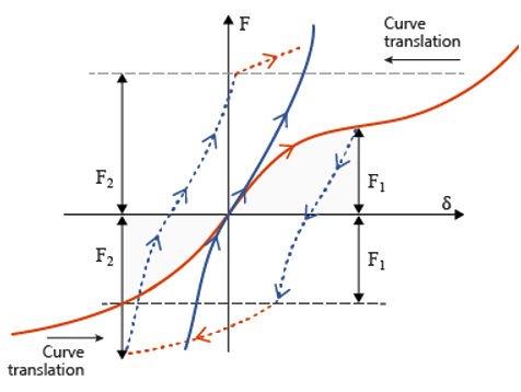
To demonstrate istropic hardening,

$H$ =1, Figure 4 shows a spring loaded in tension and then unloads using the linear unloading stiffness,

$K_{u}$ . The unloading stiffness continues to be used in compressive loading until the loading force in compression matches the maximum loading force in tension. From this point, any additional compressive loading uses the input loading function.

Nonlinear Elastic Plastic Spring with Uncoupled Hardening, H=2

The force versus displacement curve

$f_{1}$ in Figure 5 is defined in fct_ID_1i and unloading stiffness

$K_{u}$ is input using

$K_{i}$ . When uncoupled harding

$H$ =2, is used, the tensile and compression behavior are uncoupled. Thus, once the unloading reaches zero force, there is no stiffness until zero displacement and then the compressive loading follows the force displacement curve.

Figure 5. Isotropic Hardening. with

$H$ =2

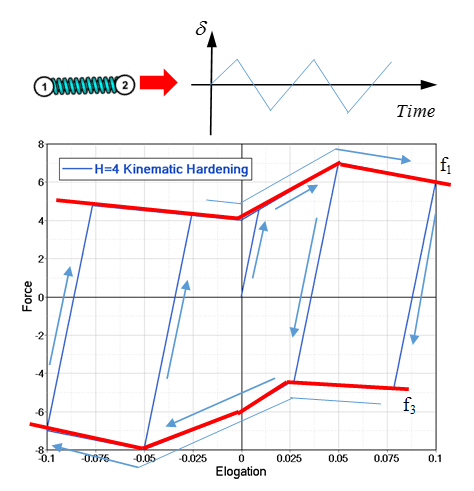
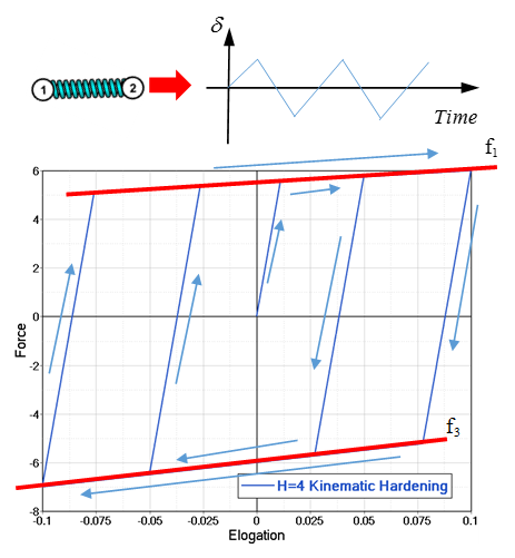
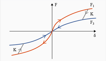
Nonlinear Elastic Plastic Spring with Kinematic Hardening, H=4

When

$H$ =4 is used, the loading function fct_ID_1i and unloading fct_ID_3i are mandatory and shown in Figure 6as

$f_{1}$ and

$f_{3}$ . The loading curve should be positive for all values of abscissa. The unloading curve in this case should be negative for all values of abscissa. These curves represents upper and lower limits of yield force as function of current spring length variation or strain. The force follows

$K$ between function

$f_{1}$ and

$f_{3}$ and is input as

$K_{i}$ .

If the minimum and maximum yield curves (

$f_{1}$ and

$f_{3}$ ) have identical shapes, the hardening is considered to be kinematic.

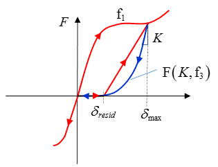
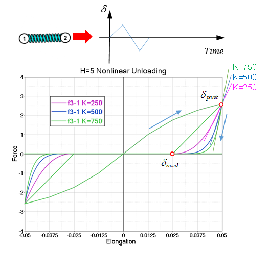
Nonlinear Elastic Plastic Spring Nonlinear Unloading, H=5

When $H$ =5, uncoupled hardening in compression and tensile with nonlinear unloading is modeled.

Function

$f_{3}$ defines the residual displacement

$δ_{r e s i d}$ related to displacement; where the unloading starts at

$δ_{p e a k}$ . The unloading is defined by: (1)

$F (K, f_{3}) = α {(δ - δ_{r e s i d})}^{n}$

with, $δ_{r e s i d} = f_{3} (δ_{p e a k})$

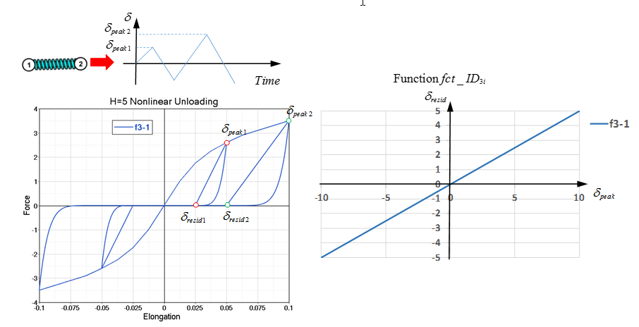
Where, α and

$n$ being computed using

$K$ and

$f_{3} (δ_{p e a k})$ . The loading function

$f_{1}$ in Figure 9 is defined in fct_ID_1i and residual deformation function

$f_{3}$ input as fct_ID_3i.

In Figure 10, a linear curve is defined for

$δ_{r e s i d}$ and

$δ_{p e a k}$ in function

$f_{3}$ .

$δ_{r e s i d}$ is 0.5 times

$δ_{p e a k}$ . In cycle loading, the first unloading started at

$δ_{p e a k 1} = 0.05$ and then

$δ_{r e s i d} = 0.5 \times 0.05 = 0.025$ . The second unloading started at

$δ_{p e a k 2} = 0.1$ and then

$δ_{r e s i d} = 0.5 \times 0.1 = 0.05$ .

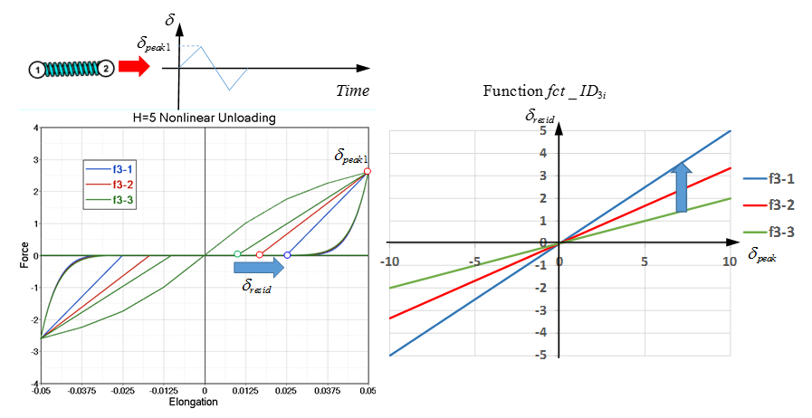
Figure 11 shows how increasing the slope of the residual versus maximum displacement curve changes the spring behavior.

Comparing Figure 10 and Figure 11, shows that the function $f_{3}$ only effects the residual displacement $δ_{r e s i d}$ and the shape of unloading curve. The shape of unloading curve is controlled by stiffness $K$ and $δ_{p e a k}$ (unloading start displacement).

If the same stiffness $K$ and same $δ_{p e a k}$ are used, then the unloading curve has the same shape.

If the same stiffness $K$ but different $δ_{p e a k}$ are used, then the unloading curve has a different shape.

If a different stiffness

$K$ and same

$δ_{p e a k}$ are used, then the unloading curve has a different shape, as shown in Figure 12.

Nonlinear Elastic Plastic Spring Istropic Hardening and Nonlinear Unloading, H=6

Both

$H$ =1 and

$H$ =6 represent isotropic hardening. In

$H$ =6, a nonlinear unloading with function

$f_{3}$ is used while

$H$ =1 uses a constant

$K_{u}$ for linear unloading. When the spring is loaded in tension and then unloads, it follows the defined unloading curve. The unloading curve continues to be used in compressive loading until the loading force in compression matches the maximum loading force in tension. From this point, additional compressive loading uses the input loading function. The loading curve in

$f_{1}$ is defined using fct_ID_1i and unloading curve in

$f_{3}$ is defined using fct_ID_3i.

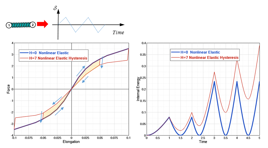
Nonlinear Elastic Plastic Spring Elastic Hysteresis, H=7

With

$H$ =7, the spring unloading is initially linear using the input

$K$ value until it reach the unloading curve

$f_{3}$ . Additional unloading follows

$f_{3}$ . If reloading occurs, the stiffness

$K$ is used to reach the curve

$f_{1}$ , which is then followed. The curve

$f_{3}$ must have ordinates smaller than curve

$f_{1}$ at a defined abscissa value. The loading curve in

$f_{1}$ is defined using fct_ID_1i and unloading curve in

$f_{3}$ is defined using fct_ID_3i.

A spring with

$H$ =7 could be used to describe hysteresis behavior. Figure 15 shows the difference between

$H$ =0 and

$H$ =7 under cycle loading. With

$H$ =0 (blue curve), it is nonlinear elastic. But with

$H$ =7 (red curve), more energy (yellow area in first loop) is absorbed, due to the hysteresis loop.

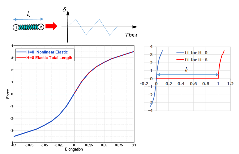
Nonlinear Elastic Total Length Function, H=8

The elastic total length spring

$H$ =8 is only available in /PROP/TYPE4. Unlike the other hardening options which use the change in spring length, this spring uses the total spring length when defining the spring stiffness. No stiffness occurs in compression. Input fct_ID_1i to define the force versus total spring length.

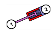
Dashpot

A dashpot (damper) can be modeled by not defining any spring stiffness. Thus, with the first term in Equation 1 removed, the force becomes only a function of the constant damping coefficient

$C_{i}$ or a nonlinear force versus velocity damping function

$h$ as fct_ID₄.(2)

$F_{i} (δ^{i}) = C_{i} {\dot{δ}}^{i} + H s c a l e_{i} h (\frac{{\dot{δ}}^{i}}{F_{i}})$

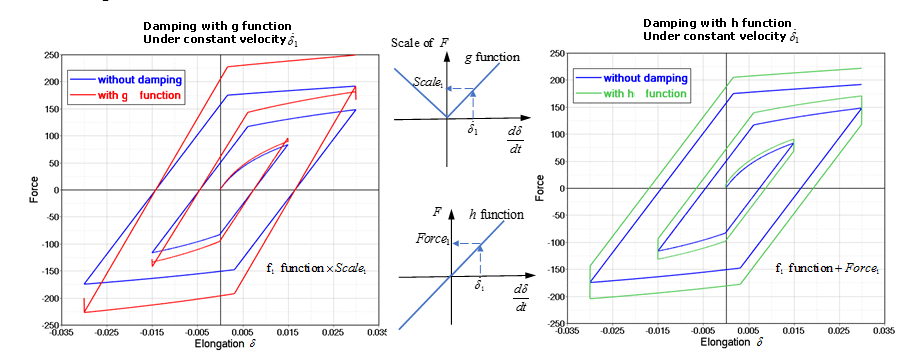
Damping Using a Function

Remembering that the $g$ function scales the force are $f_{1} \cdot g$ , whereas the $h$ function adds to the force $f_{1} + h$ . Figure 19 compares these two different methods.

A cyclic loading is applied to a nonlinear elastic plastic spring (

$H$ =1) and in two models one which uses the

$g$ function to scale the force and the other uses the

$h$ function to add to the force.

Note: The function

$h$ should have thesame sign as velocity, but the function

$g$ should be always positive, due to it is a multiplier to force displacement curve

$f_{1}$ .

Inconsistent Stiffness

When creating a spring property with a user-defined curve "Force vs Displacement" for the stiffness, typically the end of the curve has a very high slope to deal with very high compression. In this case, the following warning is often received with Radioss Starter.

WARNING ID: 506 
** WARNING IN SPRING PROPERTY
** WARNING IN SPRING PROPERTY SET ID=XXX
STIFFNESS VALUE 100 IS NOT CONSISTENT WITH THE MAXIMUM SLOPE (4550)
OF THE YIELD FUNCTION ID=X
THE STIFFNESS VALUE IS CHANGED TO 1000

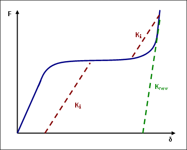
This warning comes from the fact that the slope of the input curve (the stiffness) is not consistent with the initial stiffness. If the maximum slope of the curve (the maximum stiffness) is greater than the initial stiffness, unloading in the zone of maximum slope will be false (Figure 1). To obtain proper behavior, Radioss Starter modifies the initial stiffness according to the maximum slope.