Particle Kinematics

Kinematics deals with position in space as a function of time and is often referred to as the "geometry of motion". ¹ The motion of particles may be described through the specification of both linear and angular coordinates and their time derivatives. Particle motion on straight lines is termed rectilinear motion, whereas motion on curved paths is called curvilinear motion. Although the rectilinear motion of particles and rigid bodies is well-known and used by engineers, the space curvilinear motion needs some feed-back, which is described in the following section.

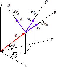
Space Curvelinear Motion

The motion of a particle along a curved path in space is called space curvilinear motion. The position vector

$R$ , the velocity

$v$ , and the acceleration of a particle along a curve are:(1)

$R = x \hat{i} + y \hat{j} + z \hat{k}$

(2)

$v = \dot{R} = \dot{x} \hat{i} + \dot{y} \hat{j} + \dot{z} \hat{k}$

(3)

$a = \ddot{R} = \ddot{x} \hat{i} + \ddot{y} \hat{j} + \ddot{z} \hat{k}$

Where

$x$ ,

$y$ and

$z$ are the coordinates of the particle and

$ \hat{i}$ ,

$\hat{j}$ and

$\hat{k}$ the unit vectors in the rectangular reference. In the cylindrical reference (

$r$ ,

$θ$ ,

$z$ ), the description of space motion calls merely for the polar coordinate expression:(4)

$v = v_{r} + v_{θ} + v_{z}$

Where,

$v_{r} = \dot{r}$

$v_{θ} = r \dot{θ}$

$v_{z} = \dot{z}$

Also, for acceleration:(5)

$a = a_{r} + a_{θ} + a_{z}$

Where,

$a_{r} = \ddot{r} - r {\dot{θ}}^{2}$

$a_{θ} = r \ddot{θ} + 2 \dot{r} \dot{θ}$

$a_{z} = \ddot{z}$

The vector location of a particle may also be described by spherical coordinates as shown in Figure 1.(6)

$v = v_{R} + v_{θ} + v_{φ}$

Where,

$v_{R} = \dot{R}$

$v_{θ} = R \dot{θ} \cos φ$

$v_{φ} = R \dot{φ}$

Using the previous expressions, the acceleration and its components can be computed:(7)

$a = a_{R} + a_{θ} + a_{φ}$

Where,

$a_{R} = \ddot{R} - R {\dot{φ}}^{2} - R {\dot{θ}}^{2} \cos^{2} φ$

$a_{θ} = \frac{\cos φ}{R} \frac{d}{d t} (R^{2} \dot{θ}) - 2 R \dot{θ} \dot{φ} \sin φ$

$a_{φ} = \frac{1}{R} \frac{d}{d t} (R^{2} \dot{φ}) + R {\dot{θ}}^{2} \sin φ \cos φ$

The choice of the coordinate system simplifies the measurement and the understanding of the problem.

Coordinate Transformation

It is frequently necessary to transform vector quantities from a given reference to another. This transformation may be accomplished with the aid of matrix algebra. The quantities to transform might be the velocity or acceleration of a particle. It could be its momentum or merely its position, considering the transformation of a velocity vector when changing from rectangular to cylindrical coordinates:(8)

${\begin{matrix} V_{r} \\ V_{θ} \\ V_{z} \end{matrix}} = [\begin{matrix} \cos θ & \sin θ & 0 \\ - \sin θ & \cos θ & 0 \\ 0 & 0 & 1 \end{matrix}] {\begin{matrix} V_{x} \\ V_{y} \\ V_{z} \end{matrix}}$

or ${V_{r θ z}} = [T_{θ}] {V_{x y z}}$

The change from cylindrical to spherical coordinates is accomplished by a single rotation

$ϕ$ of the axes around the

$θ$ -axis. The transfer matrix can be written directly from the previous equation where the rotation

$ϕ$ occurs in the

$R - ϕ$ plane:(9)

${\begin{matrix} V_{R} \\ V_{θ} \\ V_{ϕ} \end{matrix}} = [\begin{matrix} \cos ϕ & 0 & \sin ϕ \\ 0 & 1 & 0 \\ - \sin ϕ & 0 & \cos ϕ \end{matrix}] {\begin{matrix} V_{r} \\ V_{θ} \\ V_{z} \end{matrix}}$

or ${V_{R θ ϕ}} = [T_{ϕ}] {V_{r θ z}}$

Direct transfer from rectangular to spherical coordinates may be accomplished by combining Equation 8 and Equation 9:(10)

${V_{R θ ϕ}} = [T_{ϕ}] [T_{θ}] {V_{x y z}}$

with: $[T_{ϕ}] [T_{θ}] = [\begin{matrix} \cos ϕ \cos θ & \cos ϕ \sin θ & \sin ϕ \\ - \sin θ & \cos θ & 0 \\ - \sin ϕ \cos θ & - \sin ϕ \sin θ & \cos ϕ \end{matrix}]$

Reference Axes Transformation

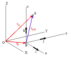
Consider now the curvilinear motion of two particles A and B in space. Study at first the translation of a reference without rotation. The motion of A is observed from a translating frame of reference x-y-z moving with the origin B (Figure 2). The position vector of A relative to B is:(11)

$r_{A / B} = x \hat{i} + y \hat{j} + z \hat{k}$

Where

$ \hat{i}$ ,

$\hat{j}$ and

$\hat{k}$ are the unit vectors in the moving x-y-z system. As there is no change of unit vectors in time, the velocity and the acceleration are derived as:(12)

$v_{A / B} = \dot{x} \hat{i} + \dot{y} \hat{j} + \dot{z} \hat{k}$

(13)

$a_{A / B} = \ddot{x} \hat{i} + \ddot{y} \hat{j} + \ddot{z} \hat{k}$

The absolute position, velocity and acceleration of

$A$ are then:(14)

$\begin{array}{l} r_{A} = r_{B} + r_{A/B} \\ v_{A} = v_{B} + v_{A/B} \\ a_{A} = a_{B} + a_{A/B} \end{array}$

In the case of rotation reference, it is proved that the angular velocity of the reference axes x-y-z may be represented by the vector:(15)

$ω = ω_{x} \hat{i} + ω_{y} \hat{j} + ω_{z} \hat{k}$

The time derivatives of the unit vectors

$ \hat{i}$ ,

$\hat{j}$ and

$\hat{k}$ due to the rotation of reference axes x-y-z about

$ω$ , can be studied by applying an infinitesimal rotation

$ω d t$ . You can write:(16)

$\frac{d}{d t} (\hat{i}) = ω \times \hat{i}; \frac{d}{d t} (\hat{j}) = ω \times \hat{j}; \frac{d}{d t} (\hat{k}) = ω \times \hat{k}$

Attention should be turned to the meaning of the time derivatives of any vector quantity

$V = V_{x} i + V_{y} j + V_{z} k$ in the rotating system. The derivative of

$V$ with respect to time as measured in the fixed frame X-Y-Z is:(17)

${(\frac{d V}{d t})}_{X Y Z} = \frac{d}{d t} (V_{x} \hat{i} + V_{y} \hat{j} + V_{z} \hat{k})$

$= (V_{x} \frac{d}{d t} (\hat{i}) + V_{y} \frac{d}{d t} (\hat{j}) + V_{z} \frac{d}{d t} (\hat{k})) + ({\dot{V}}_{x} \hat{i} + {\dot{V}}_{y} \hat{j} + {\dot{V}}_{z} \hat{k})$

With the substitution of Equation 16, the terms in the first parentheses becomes

$ω \times V$ . The terms in the second parentheses represent the components of time derivatives

${(\frac{d V}{d t})}_{x y z}$ as measured relative to the moving x-y-z reference axes. Thus:(18)

${(\frac{d V}{d t})}_{X Y Z} = ω \times V + {(\frac{d V}{d t})}_{x y z}$

This equation establishes the relation between the time derivative of a vector quantity in a fixed system and the time derivative of the vector as observed in the rotating system.

Consider now the space motion of a particle

$A$ , as observed both from a rotating system x-y-z and a fixed system X-Y-Z (Figure 3).

The origin of the rotating system coincides with the position of a second reference particle

$B$ , and the system has an angular velocity

$ω$ . Standing

$r$ for

$r_{A / B}$ , the time derivative of the vector position gives:(19)

$r_{A} = r_{B} + r \Rightarrow v_{A} = v_{B} + r$

From Equation 18

(20)

$\dot{r} = {(\frac{d r}{d t})}_{X Y Z} = ω \times r + v_{rel}$

Where,

$v_{rel}$ denotes the relative velocity measured in x-y-z, that is: (21)

$v_{rel} = {(d r/dt)}_{x y z} = \dot{x} \hat{i} + \dot{y} \hat{j} + \dot{z} \hat{k}$

Thus, the relative velocity equation becomes:(22)

$v_{A} = v_{B} + ω \times r + v_{rel}$

The relative acceleration equation is the time derivative of Equation 22 which gives:(23)

$a_{A} = a_{B} + \dot{ω} \times r + ω \times \dot{r} + {\dot{v}}_{rel}$

Where, the last term can be obtained from Equation 18:(24)

${\dot{v}}_{rel} = {(\frac{d v_{rel}}{d t})}_{X Y Z} = ω \times v_{rel} + a_{rel}$

and (25)

$a_{rel} = {(\frac{d v_{rel}}{d t})}_{x y z} = \ddot{x} \hat{i} + \ddot{y} \hat{j} + \ddot{z} \hat{k}$

Combining Equation 23 to Equation 25, you obtain upon collection of terms:(26)

$a_{A} = a_{B} + \dot{ω} \times r + ω \times (ω \times r) + 2 ω \times v_{rel} + a_{rel}$

Where, the term $2 ω \times v_{rel}$ constitutes Coriolis acceleration.

Skew and Frame Notations

Two kinds of reference definition are available in Radioss:

Skew Reference: A projection reference to define the local quantities with respect to the global reference. In fact the origin of skew remains at the initial position during the motion even though a moving skew is defined. In this case, a simple projection matrix is used to compute the kinematic quantities in the reference.
Frame Reference: A mobile or fixed reference. The quantities are computed with respect to the origin of the frame which may be in motion or not depending to the kind of reference frame. For a moving reference frame, the position and the orientation of the reference vary in time during the motion. The origin of the frame defined by a node position is tied to the node. Equation 22 and Equation 26 are used to compute the accelerations and velocities in the frame.

Meriam J.L., “Dynamics”, John Wiley & Sons, Second edition, 1975.