Moving Least Squares Method (MLSM)

Builds a weighted least squares model where the weights associated with the sampling points do not remain constant.

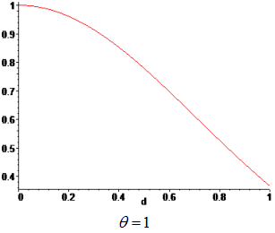
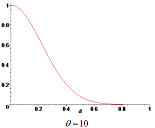
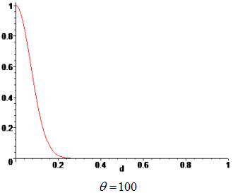
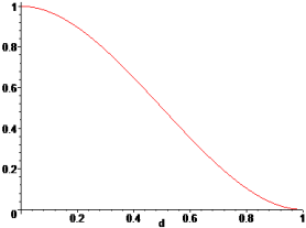
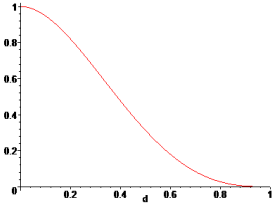
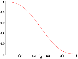
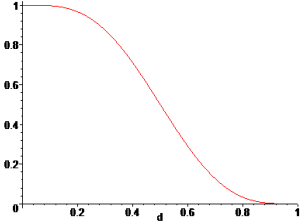
Weights are functions of the normalized distance from a sampling point to a point x, where the surrogate model is evaluated. The weight, associated to a sampling point, decays as the evaluation point moves away from it. The decay is defined through a decay function. For each point x it reconstructs a continuous function biased towards the region around that point.

Usability Characteristics

Suggested to be used for nonlinear and noisy output responses.
Residuals and diagnostics should be used to gain an understanding of the quality of the Fit.
Use a Testing matrix in addition to an Input matrix for better diagnostics.
Quality of a Moving Least Squares Method Fit is a function of the number of runs, order of the polynomial and the behavior of the application.
If the residuals and diagnostics are not good for a Moving Least Squares Method Fit, than you can increase the order of the Fit provided you have enough runs to fit that specific order.
Because the weights are not constant in Moving Least Squares Method, there is no analytical form and an equation can not be provided.

Settings

In the Specifications step, Settings tab, change method settings.

Note: For most applications the default settings work optimally, and you may only need to change the Order to improve the Fit quality.

Parameter	Default	Range	Description
Fit Parameter	5.0	>= 0.0 <= 10.0	Controls the effect of screening out noise; the larger value, the less effect.
Minimum Weight	0.001	> 0.0	Minimum weight.
Number of Excess Points	3	>=0	Number of excessive points to build Moving Least Squares Method.
Regression Model	Linear	Linear Squared Cubic Interaction Full Quadratic Full Cubic Custom	Order of polynomial function.
Weighting Function	Gaussian	Gaussian (Recommended) Cubic Fourth Order Fifth Order Seventh Order	Type of weighting function. Gaussian $W_{i} = \exp (- θ r_{i}^{2})$ where $r_{i}$ is the normalized distance from the i-th sampling point to a current point. The parameter $θ$ defines the "closeness of fit", the case $θ$ =0 is equivalent to the traditional Least Squares Regression. When the parameter $θ$ is large, it is possible to obtain a very close fit through the sampling points, if desired. The images in Figure 1 illustrate the change of the weight over the interval [0,1] where the sampling point is at r = 0. Figure 1. Cubic $w_{i} = 1 - 3 p_{i}^{2} + 2 p_{i}^{3}$ where $p_{i} = r_{i} / R_{\max}, R_{\max}$ is the normalized radius of the sphere of influence. Figure 2. The normalized radius of the sphere of influence $R_{\max}$ inversely relates to the closeness of fit parameter, for example the smaller the value of $R_{\max}$ , the closer fit is obtained. Fourth Order $w_{i} = 1 - 6 p_{i}^{2} + 8 p_{i}^{3} + 3 p_{i}^{4}$ Figure 3. Fifth Order $w_{i} = 1 - 10 p_{i}^{3} + 15 p_{i}^{4} + 6 p_{i}^{5}$ Figure 4. Seventh Order $w_{i} = 1 - 35 p_{i}^{4} + 84 p_{i}^{5} + 70 p_{i}^{6} + 20 p_{i}^{7}$ Figure 5.