The file graphic type is used when realistic shapes of the bodies of the mechanism
are to be included in the model.
File graphics can be imported into MotionView using the Import CAD
or FE using HyperMesh utility, or if an H3D file of the
CAD data already exists then it can be manually added (using the method described
below). Other file formats that are supported include: .fem,
.shl, .obj, and
.g.
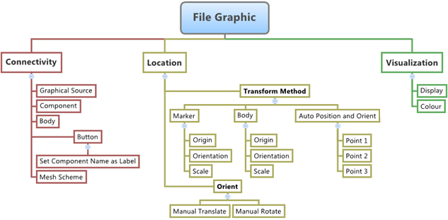
The figure below shows the various file graphic options and settings that are
available in MotionView:
Figure 1.
If the Graphics panel is not currently displayed, select the desired graphic by
clicking on it in the Project Browser or in the modeling window.
The Graphics panel is automatically displayed.
Use the icon next to Graphic source to browse and select a graphic file.
Click the Body collector and
select a body from the modeling window, or double click
the Body collector to open the Model Tree (from which the desired body can be selected).
Use the Component drop-down menu (located in the top right corner of the panel)
to select All or the desired component name.
Click the Set Label to Component
Name button to set the component name as the label of the
graphic entity.
Use the Mesh Scheme drop-down menu to control the level of discretization of
the graphic written to the solver deck.
Controlling the mesh scheme is useful in reducing the size of the solver deck
as well as result files, when the mesh does not influence the solution.
Option
Description
Aggressive
Reduces the most resolution from the triamesh.
Average
Reduces some resolution from the triamesh.
Conservative
Reduces the resolution of the trimesh slightly.
None
This option does not change the resolution of the triamesh.
Tip: This setting is recommended if the graphic is used in
contacts.
When the MotionView model is exported to MotionSolve, the file graphic information is written as a
triangular mesh with nodes and elements (tessellation). A fine mesh on the
surfaces results in a large amount of nodes and elements in the MotionSolve XML file and subsequently a larger size
MotionSolve results animation file. The Mesh
Scheme setting provides a way to coarsen the mesh upon export, thus reducing the
file size of the XML as much as possible.
Click the Location tab.
If the imported H3D file graphic is not positioned/oriented in the desired
fashion in the model reference frame, this can be corrected using the options
available on the Location tab.
Select a transformation method from the Transform Method drop-down menu.
If Marker is chosen:
Click the Marker collector and select the marker
that you want to use as a reference marker for transformation.
By default the global frame is set as the reference marker.
If you know the absolute values of the position and orientation of the
graphic with respect to the chosen reference marker, enter those values
in the X, Y, Z fields (located under Origin) and the three Euler angles
(in radians) in the three Orientation fields.
If you do not know the absolute values of position and orientation,
incrementally move and rotate the graphic by clicking
Orient and invoking the Graphic
Orient dialog.
Enter the desired translational displacement values in the fields
labeled Translate (for any or all of the three translational axes) by
clicking the appropriate check box. Click the +
or – buttons for the graphic to be moved
accordingly.
In the fields labeled Rotate, click the desired radio button for
RX, RY, or
RZ and enter the desired rotation value in
degrees. Click the + or –
buttons to apply the rotation.
Repeat the same process for the other two rotational axes if
required.
Click OK to close the dialog.
The entered values will now be applied to the graphic and will
be displayed on the panel.
Under Scale, enter three scaling factors for the
graphic object in the Cartesian directions.
If Body is chosen:
Click the Body collector and select the body to
be used as a reference for specifying the location and orientation for
the file graphic.
Use the same steps as described in the marker transformation method to
locate and orient the graphic.
Note: If the CAD or FE Import utility was used to import the graphic
into the model and if locator points were created to specify the
three points on the graphic, then three additional transform methods
are available:
Auto Position
Auto Position and Orient
Auto Position, Orient and Scale
As the names suggest, the three methods use the three locator points
to position and orient and/or scale the imported file graphic.
If Auto Position is chosen:
Click the Point 1 collector and pick a point
from the modeling window (or the Model Tree) that represents the position of the file
graphic.
Enter the orientation and scale values for the file graphic in their
respective fields.
If Auto Position and Orient is chosen:
Click the Point 1 collector and pick a point
from the modeling window (or the Model Tree) that represents the position of the file
graphic.
Select a point that represents the orientation of the graphic for the
Point 2 collector.
Enter three scale values in the fields labeled Scale.
If Auto Position, Orient and Scale is chosen, select
the three points that represent the position (Point 1), orientation (Point 2),
and scale (Point 3) of the file graphic and the graphic will be automatically
moved to desired location with proper orientation and scale.
Click the Inertia Properties
tab and review the mass and center of mass coordinates for the graphic.