Uniaxial Fatigue Analysis

Uniaxial Fatigue Analysis, using S-N (stress-life) and E-N (strain-life) approaches for predicting the life (number of loading cycles) of a structure under cyclical loading may be performed by using HyperLife.

The stress-life method works well in predicting fatigue life when the stress level in the structure falls mostly in the elastic range. Under such cyclical loading conditions, the structure typically can withstand a large number of loading cycles; this is known as high-cycle fatigue. When the cyclical strains extend into plastic strain range, the fatigue endurance of the structure typically decreases significantly; this is characterized as low-cycle fatigue. The generally accepted transition point between high-cycle and low-cycle fatigue is around 10,000 loading cycles. For low-cycle fatigue prediction, the strain-life (E-N) method is applied, with plastic strains being considered as an important factor in the damage calculation.

Stress-Life (S-N) Approach

S-N Curve

The S-N curve, first developed by Wöhler, defines a relationship between stress and number of cycles to failure. Typically, the S-N curve (and other fatigue properties) of a material is obtained from experiment; through fully reversed rotating bending tests. Due to the large amount of scatter that usually accompanies test results, statistical characterization of the data should also be provided (certainty of survival is used to modify the S-N curve according to the standard error of the curve and a higher reliability level requires a larger certainty of survival).


Figure 1. S-N Data from Testing
When S-N testing data is presented in a log-log plot of alternating nominal stress amplitude S a or range S R versus cycles to failure N , the relationship between S and N can be described by straight line segments. Normally, a one or two segment idealization is used.


Figure 2. One Segment S-N Curves in Log-Log Scale
(1) S = S 1 ( N f ) b 1

for segment 1

Where, S is the nominal stress range, N f are the fatigue cycles to failure, b l is the first fatigue strength exponent, and S I is the fatigue strength coefficient.

The S-N approach is based on elastic cyclic loading, inferring that the S-N curve should be confined, on the life axis, to numbers greater than 1000 cycles. This ensures that no significant plasticity is occurring. This is commonly referred to as high-cycle fatigue.

S-N curve data is provided for a given material using the Materials module.

Rainflow Cycle Counting

Cycle counting is used to extract discrete simple "equivalent" constant amplitude cycles from a random loading sequence. One way to understand "cycle counting" is as a changing stress-strain versus time signal. Cycle counting will count the number of stress-strain hysteresis loops and keep track of their range/mean or maximum/minimum values.

Rainflow cycle counting is the most widely used cycle counting method. It requires that the stress time history be rearranged so that it contains only the peaks and valleys and it starts either with the highest peak or the lowest valley (whichever is greater in absolute magnitude). Then, three consecutive stress points (1, 2, and 3) will define two consecutive ranges as Δ S 12 = | S 1 S 2 | MathType@MTEF@5@5@+= feaagKart1ev2aaatCvAUfeBSjuyZL2yd9gzLbvyNv2CaerbuLwBLn hiov2DGi1BTfMBaeXatLxBI9gBaerbd9wDYLwzYbItLDharqqtubsr 4rNCHbGeaGqiVu0Je9sqqrpepC0xbbL8F4rqqrFfpeea0xe9Lq=Jc9 vqaqpepm0xbba9pwe9Q8fs0=yqaqpepae9pg0FirpepeKkFr0xfr=x fr=xb9adbaqaaeGaciGaaiaabeqaamaabaabaaGcbaGaeyiLdqKaam 4uamaaBaaaleaacaaIXaGaaGOmaaqabaGccqGH9aqpdaabdaqaaiaa dofadaWgaaWcbaGaaGymaaqabaGccqGHsislcaWGtbWaaSbaaSqaai aaikdaaeqaaaGccaGLhWUaayjcSdaaaa@428A@ and Δ S 23 = | S 2 S 3 | MathType@MTEF@5@5@+= feaagKart1ev2aqatCvAUfeBSjuyZL2yd9gzLbvyNv2CaerbuLwBLn hiov2DGi1BTfMBaeXatLxBI9gBaerbd9wDYLwzYbItLDharqqtubsr 4rNCHbGeaGqiVu0Je9sqqrpepC0xbbL8F4rqqrFfpeea0xe9Lq=Jc9 vqaqpepm0xbba9pwe9Q8fs0=yqaqpepae9pg0FirpepeKkFr0xfr=x fr=xb9adbaqaaeGaciGaaiaabeqaamaabaabaaGcbaGaeyiLdqKaam 4uamaaBaaaleaacaaIYaGaaG4maaqabaGccqGH9aqpdaabdaqaaiaa dofadaWgaaWcbaGaaGOmaaqabaGccqGHsislcaWGtbWaaSbaaSqaai aaiodaaeqaaaGccaGLhWUaayjcSdaaaa@428F@ |. A cycle from 1 to 2 is only extracted if Δ S 12 Δ S 23 MathType@MTEF@5@5@+= feaagKart1ev2aqatCvAUfeBSjuyZL2yd9gzLbvyNv2CaerbuLwBLn hiov2DGi1BTfMBaeXatLxBI9gBaerbd9wDYLwzYbItLDharqqtubsr 4rNCHbGeaGqiVu0Je9sqqrpepC0xbbL8F4rqqrFfpeea0xe9Lq=Jc9 vqaqpepm0xbba9pwe9Q8fs0=yqaqpepae9pg0FirpepeKkFr0xfr=x fr=xb9adbaqaaeGaciGaaiaabeqaamaabaabaaGcbaGaeyiLdqKaam 4uamaaBaaaleaacaaIXaGaaGOmaaqabaGccqGHKjYOcqGHuoarcaWG tbWaaSbaaSqaaiaaikdacaaIZaaabeaaaaa@3F7C@ . Once a cycle is extracted, the two points forming the cycle are discarded and the remaining points are connected to each other. This procedure is repeated until the remaining data points are exhausted.
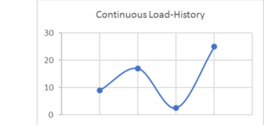
  • Simple Load History:


    Figure 3. Continuous Load History
    Since this load history is continuous, it is converted into a load history consisting of peaks and valleys only.
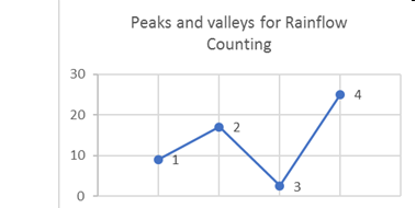

    Figure 4. Peaks and Valleys for Rainflow Counting. 1, 2, 3, and 4 are the four peaks and valleys
    It is clear that point 4 is the peak stress in the load history, and it will be moved to the front during rearrangement (Figure 5). After rearrangement, the peaks and valleys are renumbered for convenience.
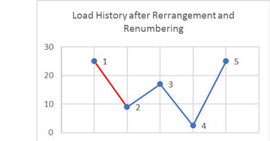

    Figure 5. Load History after Rearrangement and Renumbering

    Next, pick the first three stress values (1, 2, and 3) and determine if a cycle is present.

    If S i MathType@MTEF@5@5@+= feaagKart1ev2aqatCvAUfeBSjuyZL2yd9gzLbvyNv2CaerbuLwBLn hiov2DGi1BTfMBaeXatLxBI9gBaerbd9wDYLwzYbItLDharqqtubsr 4rNCHbGeaGqiVu0Je9sqqrpepC0xbbL8F4rqqrFfpeea0xe9Lq=Jc9 vqaqpepm0xbba9pwe9Q8fs0=yqaqpepae9pg0FirpepeKkFr0xfr=x fr=xb9adbaqaaeGaciGaaiaabeqaamaabaabaaGcbaGaam4uamaaBa aaleaacaWGPbaabeaaaaa@37E9@ represents the stress value, point i MathType@MTEF@5@5@+= feaagKart1ev2aqatCvAUfeBSjuyZL2yd9gzLbvyNv2CaerbuLwBLn hiov2DGi1BTfMBaeXatLxBI9gBaerbd9wDYLwzYbItLDharqqtubsr 4rNCHbGeaGqiVu0Je9sqqrpepC0xbbL8F4rqqrFfpeea0xe9Lq=Jc9 vqaqpepm0xbba9pwe9Q8fs0=yqaqpepae9pg0FirpepeKkFr0xfr=x fr=xb9adbaqaaeGaciGaaiaabeqaamaabaabaaGcbaWaaSbaaSqaai aadMgaaeqaaaaa@3711@ then:(2) Δ S 12 = | S 1 S 2 | MathType@MTEF@5@5@+= feaagKart1ev2aaatCvAUfeBSjuyZL2yd9gzLbvyNv2CaerbuLwBLn hiov2DGi1BTfMBaeXatLxBI9gBaerbd9wDYLwzYbItLDharqqtubsr 4rNCHbGeaGqiVu0Je9sqqrpepC0xbbL8F4rqqrFfpeea0xe9Lq=Jc9 vqaqpepm0xbba9pwe9Q8fs0=yqaqpepae9pg0FirpepeKkFr0xfr=x fr=xb9adbaqaaeGaciGaaiaabeqaamaabaabaaGcbaGaeyiLdqKaam 4uamaaBaaaleaacaaIXaGaaGOmaaqabaGccqGH9aqpdaabdaqaaiaa dofadaWgaaWcbaGaaGymaaqabaGccqGHsislcaWGtbWaaSbaaSqaai aaikdaaeqaaaGccaGLhWUaayjcSdaaaa@428A@ (3) Δ S 23 = | S 2 S 3 | MathType@MTEF@5@5@+= feaagKart1ev2aqatCvAUfeBSjuyZL2yd9gzLbvyNv2CaerbuLwBLn hiov2DGi1BTfMBaeXatLxBI9gBaerbd9wDYLwzYbItLDharqqtubsr 4rNCHbGeaGqiVu0Je9sqqrpepC0xbbL8F4rqqrFfpeea0xe9Lq=Jc9 vqaqpepm0xbba9pwe9Q8fs0=yqaqpepae9pg0FirpepeKkFr0xfr=x fr=xb9adbaqaaeGaciGaaiaabeqaamaabaabaaGcbaGaeyiLdqKaam 4uamaaBaaaleaacaaIYaGaaG4maaqabaGccqGH9aqpdaabdaqaaiaa dofadaWgaaWcbaGaaGOmaaqabaGccqGHsislcaWGtbWaaSbaaSqaai aaiodaaeqaaaGccaGLhWUaayjcSdaaaa@428F@
    As you can see from Figure 5 , Δ S 12 Δ S 23 MathType@MTEF@5@5@+= feaagKart1ev2aqatCvAUfeBSjuyZL2yd9gzLbvyNv2CaerbuLwBLn hiov2DGi1BTfMBaeXatLxBI9gBaerbd9wDYLwzYbItLDharqqtubsr 4rNCHbGeaGqiVu0Je9sqqrpepC0xbbL8F4rqqrFfpeea0xe9Lq=Jc9 vqaqpepm0xbba9pwe9Q8fs0=yqaqpepae9pg0FirpepeKkFr0xfr=x fr=xb9adbaqaaeGaciGaaiaabeqaamaabaabaaGcbaGaeyiLdqKaam 4uamaaBaaaleaacaaIXaGaaGOmaaqabaGccqGHLjYScqGHuoarcaWG tbWaaSbaaSqaaiaaikdacaaIZaaabeaaaaa@3F8D@ ; therefore, no cycle is extracted from point 1 to 2. Now consider the next three points (2, 3, and 4).(4) Δ S 23 = | S 2 S 3 | MathType@MTEF@5@5@+= feaagKart1ev2aqatCvAUfeBSjuyZL2yd9gzLbvyNv2CaerbuLwBLn hiov2DGi1BTfMBaeXatLxBI9gBaerbd9wDYLwzYbItLDharqqtubsr 4rNCHbGeaGqiVu0Je9sqqrpepC0xbbL8F4rqqrFfpeea0xe9Lq=Jc9 vqaqpepm0xbba9pwe9Q8fs0=yqaqpepae9pg0FirpepeKkFr0xfr=x fr=xb9adbaqaaeGaciGaaiaabeqaamaabaabaaGcbaGaeyiLdqKaam 4uamaaBaaaleaacaaIYaGaaG4maaqabaGccqGH9aqpdaabdaqaaiaa dofadaWgaaWcbaGaaGOmaaqabaGccqGHsislcaWGtbWaaSbaaSqaai aaiodaaeqaaaGccaGLhWUaayjcSdaaaa@428F@ (5) Δ S 34 = | S 3 S 4 | MathType@MTEF@5@5@+= feaagKart1ev2aqatCvAUfeBSjuyZL2yd9gzLbvyNv2CaerbuLwBLn hiov2DGi1BTfMBaeXatLxBI9gBaerbd9wDYLwzYbItLDharqqtubsr 4rNCHbGeaGqiVu0Je9sqqrpepC0xbbL8F4rqqrFfpeea0xe9Lq=Jc9 vqaqpepm0xbba9pwe9Q8fs0=yqaqpepae9pg0FirpepeKkFr0xfr=x fr=xb9adbaqaaeGaciGaaiaabeqaamaabaabaaGcbaGaeyiLdqKaam 4uamaaBaaaleaacaaIYaGaaG4maaqabaGccqGH9aqpdaabdaqaaiaa dofadaWgaaWcbaGaaGOmaaqabaGccqGHsislcaWGtbWaaSbaaSqaai aaiodaaeqaaaGccaGLhWUaayjcSdaaaa@428F@
    Δ S 23 Δ S 34 MathType@MTEF@5@5@+= feaagKart1ev2aqatCvAUfeBSjuyZL2yd9gzLbvyNv2CaerbuLwBLn hiov2DGi1BTfMBaeXatLxBI9gBaerbd9wDYLwzYbItLDharqqtubsr 4rNCHbGeaGqiVu0Je9sqqrpepC0xbbL8F4rqqrFfpeea0xe9Lq=Jc9 vqaqpepm0xbba9pwe9Q8fs0=yqaqpepae9pg0FirpepeKkFr0xfr=x fr=xb9adbaqaaeGaciGaaiaabeqaamaabaabaaGcbaGaeyiLdqKaam 4uamaaBaaaleaacaaIYaGaaG4maaqabaGccqGHKjYOcqGHuoarcaWG tbWaaSbaaSqaaiaaiodacaaI0aaabeaaaaa@3F80@ , hence a cycle is extracted from point 2 to 3. Now that a cycle has been extracted, the two points are deleted from the graph.
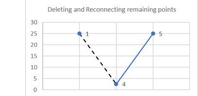

    Figure 6. Delete and Reconnect Remaining Points
    The same process is applied to the remaining points:(6) Δ S 14 = | S 1 S 4 | MathType@MTEF@5@5@+= feaagKart1ev2aqatCvAUfeBSjuyZL2yd9gzLbvyNv2CaerbuLwBLn hiov2DGi1BTfMBaeXatLxBI9gBaerbd9wDYLwzYbItLDharqqtubsr 4rNCHbGeaGqiVu0Je9sqqrpepC0xbbL8F4rqqrFfpeea0xe9Lq=Jc9 vqaqpepm0xbba9pwe9Q8fs0=yqaqpepae9pg0FirpepeKkFr0xfr=x fr=xb9adbaqaaeGaciGaaiaabeqaamaabaabaaGcbaGaeyiLdqKaam 4uamaaBaaaleaacaaIYaGaaG4maaqabaGccqGH9aqpdaabdaqaaiaa dofadaWgaaWcbaGaaGOmaaqabaGccqGHsislcaWGtbWaaSbaaSqaai aaiodaaeqaaaGccaGLhWUaayjcSdaaaa@428F@ (7) Δ S 45 = | S 4 S 5 | MathType@MTEF@5@5@+= feaagKart1ev2aqatCvAUfeBSjuyZL2yd9gzLbvyNv2CaerbuLwBLn hiov2DGi1BTfMBaeXatLxBI9gBaerbd9wDYLwzYbItLDharqqtubsr 4rNCHbGeaGqiVu0Je9sqqrpepC0xbbL8F4rqqrFfpeea0xe9Lq=Jc9 vqaqpepm0xbba9pwe9Q8fs0=yqaqpepae9pg0FirpepeKkFr0xfr=x fr=xb9adbaqaaeGaciGaaiaabeqaamaabaabaaGcbaGaeyiLdqKaam 4uamaaBaaaleaacaaIYaGaaG4maaqabaGccqGH9aqpdaabdaqaaiaa dofadaWgaaWcbaGaaGOmaaqabaGccqGHsislcaWGtbWaaSbaaSqaai aaiodaaeqaaaGccaGLhWUaayjcSdaaaa@428F@

    In this case, Δ S 14 = Δ S 45 MathType@MTEF@5@5@+= feaagKart1ev2aqatCvAUfeBSjuyZL2yd9gzLbvyNv2CaerbuLwBLn hiov2DGi1BTfMBaeXatLxBI9gBaerbd9wDYLwzYbItLDharqqtubsr 4rNCHbGeaGqiVu0Je9sqqrpepC0xbbL8F4rqqrFfpeea0xe9Lq=Jc9 vqaqpepm0xbba9pwe9Q8fs0=yqaqpepae9pg0FirpepeKkFr0xfr=x fr=xb9adbaqaaeGaciGaaiaabeqaamaabaabaaGcbaGaeyiLdqKaam 4uamaaBaaaleaacaaIXaGaaGinaaqabaGccqGH9aqpcqGHuoarcaWG tbWaaSbaaSqaaiaaisdacaaI1aaabeaaaaa@3ED3@ , so another cycle is extracted from point 1 to 4. After these two points are also discarded, only point 5 remains; therefore, the rainflow counting process is completed.

    Two cycles (2→3 and 1→4) have been extracted from this load history. One of the main reasons for choosing the highest peak/valley and rearranging the load history is to guarantee that the largest cycle is always extracted (in this case, it is 1→4). If you observe the load history prior to rearrangement, and conduct the same rainflow counting process on it, then clearly, the 1→4 cycle is not extracted.

  • Complex Load History
    The rainflow counting process is the same regardless of the number of load history points. However, depending on the location of the highest peak/valley used for rearrangement, it may not be obvious how the rearrangement process is conducted. Figure 7 shows just the rearrangement process for a more complex load history. The subsequent rainflow counting is just an extrapolation of the process mentioned in the simple example above, and is not repeated here.
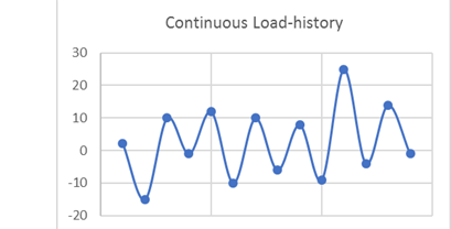

    Figure 7. Continuous Load History
    Since this load history is continuous, it is converted into a load history consisting of peaks and valleys only:
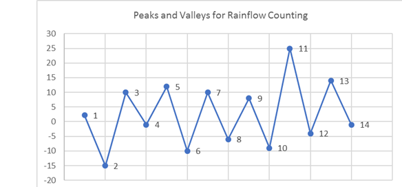

    Figure 8. Peaks and Valleys for Rainflow Counting
    Clearly, load point 11 is the highest valued load and therefore, the load history is now rearranged and renumbered.
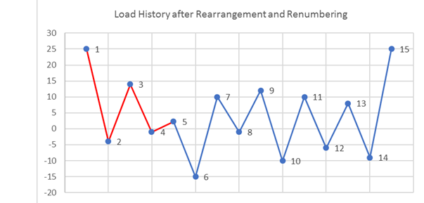

    Figure 9. Load History After Rearrangement and Renumbering

    The load history is rearranged such that all points including and after the highest load are moved to the beginning of the load history and are removed from the end of the load history.

Equivalent Nominal Stress

Since S-N theory deals with uniaxial stress, the stress components need to be resolved into one combined value for each calculation point, at each time step, and then used as equivalent nominal stress applied on the S-N curve.

Various stress combination types are available with the default being "Absolute maximum principle stress". "Absolute maximum principle stress" is recommended for brittle materials, while "Signed von Mises stress" is recommended for ductile material. The sign on the signed parameters is taken from the sign of the Maximum Absolute Principal value.

Mean Stress Correction

Generally, S-N curves are obtained from standard experiments with fully reversed cyclic loading. However, the real fatigue loading could not be fully-reversed, and the normal mean stresses have significant effect on fatigue performance of components. Tensile normal mean stresses are detrimental and compressive normal mean stresses are beneficial, in terms of fatigue strength. Mean stress correction is used to take into account the effect of non-zero mean stresses.

The Gerber parabola and the Goodman line in Haigh's coordinates are widely used when considering mean stress influence, and can be expressed as:

Gerber:(8) S e = S r ( 1 ( S m S u ) 2 )
Goodman:(9) S e = S r ( 1 S m S u )
Where,
S m
Mean stress given by S m = ( S m a x + S m i n ) / 2
S r
Stress Range given by S r = S m a x S m i n
S e
Stress range after mean stress correction (for a stress range S r and a mean stress S m )
S u
Ultimate strength

The Gerber method treats positive and negative mean stress correction in the same way that mean stress always accelerates fatigue failure, while the Goodman method ignores the negative means stress. Both methods give conservative result for compressive means stress. The Goodman method is recommended for brittle material while the Gerber method is recommended for ductile material. For the Goodman method, if the tensile means stress is greater than UTS, the damage will be greater than 1.0. For the Gerber method, if the mean stress is greater than UTS, the damage will be greater than 1.0, with either tensile or compressive.

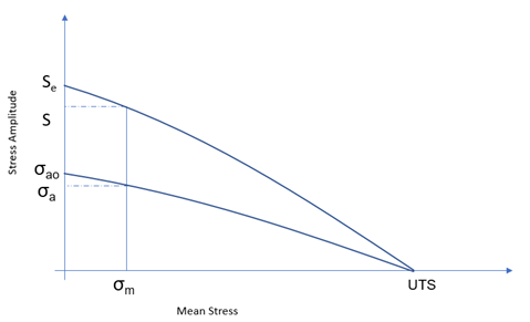
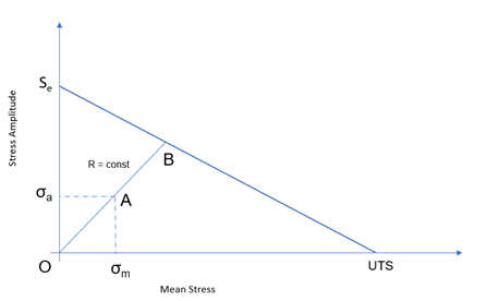
A Haigh diagram characterizes different combinations of stress amplitude and mean stress for a given number of cycles to failure.


Figure 10. Haigh Diagram and Mean Stress Correction Methods

Parameters affecting mean stress influence can be defined using the mean stress correction in the Fatigue Module dialog and the Assign Material dialog.

GERBER2:

Improves the Gerber method by ignoring the effect of negative mean stress.

SODERBERG:

Is slightly different from GOODMAN; the mean stress is normalized by yield stress instead of ultimate tensile stress.(10) S e = S a ( 1 S m S y ) MathType@MTEF@5@5@+= feaagKart1ev2aqatCvAUfeBSjuyZL2yd9gzLbvyNv2CaerbuLwBLn hiov2DGi1BTfMBaeXatLxBI9gBaerbd9wDYLwzYbItLDharqqtubsr 4rNCHbGeaGqiVu0Je9sqqrpepC0xbbL8F4rqqrFfpeea0xe9Lq=Jc9 vqaqpepm0xbba9pwe9Q8fs0=yqaqpepae9pg0FirpepeKkFr0xfr=x fr=xb9adbaqaaeGaciGaaiaabeqaamaabaabaaGcbaGaam4uamaaBa aaleaacaWGLbaabeaakiabg2da9maalaaabaGaam4uamaaBaaaleaa caWGHbaabeaaaOqaamaabmaabaGaaGymaiabgkHiTmaalaaabaGaam 4uamaaBaaaleaacaWGTbaabeaaaOqaaiaadofadaWgaaWcbaGaamyE aaqabaaaaaGccaGLOaGaayzkaaaaaaaa@4246@
Where,
S e MathType@MTEF@5@5@+= feaagKart1ev2aqatCvAUfeBSjuyZL2yd9gzLbvyNv2CaerbuLwBLn hiov2DGi1BTfMBaeXatLxBI9gBaerbd9wDYLwzYbItLDharqqtubsr 4rNCHbGeaGqiVu0Je9sqqrpepC0xbbL8F4rqqrFfpeea0xe9Lq=Jc9 vqaqpepm0xbba9pwe9Q8fs0=yqaqpepae9pg0FirpepeKkFr0xfr=x fr=xb9adbaqaaeGaciGaaiaabeqaamaabaabaaGcbaGaam4uamaaBa aaleaacaWGLbaabeaaaaa@37E5@
Equivalent stress amplitude
S a MathType@MTEF@5@5@+= feaagKart1ev2aqatCvAUfeBSjuyZL2yd9gzLbvyNv2CaerbuLwBLn hiov2DGi1BTfMBaeXatLxBI9gBaerbd9wDYLwzYbItLDharqqtubsr 4rNCHbGeaGqiVu0Je9sqqrpepC0xbbL8F4rqqrFfpeea0xe9Lq=Jc9 vqaqpepm0xbba9pwe9Q8fs0=yqaqpepae9pg0FirpepeKkFr0xfr=x fr=xb9adbaqaaeGaciGaaiaabeqaamaabaabaaGcbaGaam4uamaaBa aaleaacaWGHbaabeaaaaa@37E1@
Stress amplitude
S m MathType@MTEF@5@5@+= feaagKart1ev2aqatCvAUfeBSjuyZL2yd9gzLbvyNv2CaerbuLwBLn hiov2DGi1BTfMBaeXatLxBI9gBaerbd9wDYLwzYbItLDharqqtubsr 4rNCHbGeaGqiVu0Je9sqqrpepC0xbbL8F4rqqrFfpeea0xe9Lq=Jc9 vqaqpepm0xbba9pwe9Q8fs0=yqaqpepae9pg0FirpepeKkFr0xfr=x fr=xb9adbaqaaeGaciGaaiaabeqaamaabaabaaGcbaGaam4uamaaBa aaleaacaWGTbaabeaaaaa@37ED@
Mean stress
S y MathType@MTEF@5@5@+= feaagKart1ev2aqatCvAUfeBSjuyZL2yd9gzLbvyNv2CaerbuLwBLn hiov2DGi1BTfMBaeXatLxBI9gBaerbd9wDYLwzYbItLDharqqtubsr 4rNCHbGeaGqiVu0Je9sqqrpepC0xbbL8F4rqqrFfpeea0xe9Lq=Jc9 vqaqpepm0xbba9pwe9Q8fs0=yqaqpepae9pg0FirpepeKkFr0xfr=x fr=xb9adbaqaaeGaciGaaiaabeqaamaabaabaaGcbaGaam4uamaaBa aaleaacaWG5baabeaaaaa@37F9@
Yield stress

FKM:

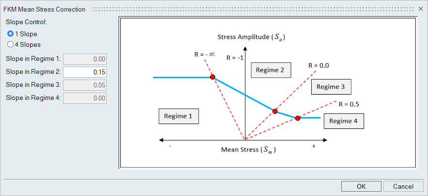
If only one slope field is specified for mean stress correction, the corresponding Mean Stress Sensitivity value ( M MathType@MTEF@5@5@+= feaagKart1ev2aqatCvAUfeBSjuyZL2yd9gzLbvyNv2CaerbuLwBLn hiov2DGi1BTfMBaeXatLxBI9gBaerbd9wDYLwzYbItLDharqqtubsr 4rNCHbGeaGqiVu0Je9sqqrpepC0xbbL8F4rqqrFfpeea0xe9Lq=Jc9 vqaqpepm0xbba9pwe9Q8fs0=yqaqpepae9pg0FirpepeKkFr0xfr=x fr=xb9adbaqaaeGaciGaaiaabeqaamaabaabaaGcbaGaamytaaaa@36C9@ ) for Mean Stress Correction is set equal to Slope in Regime 2 (Figure 11). Based on FKM-Guidelines, the Haigh diagram is divided into four regimes based on the Stress ratio ( R = S min / S max MathType@MTEF@5@5@+= feaagKart1ev2aaatCvAUfeBSjuyZL2yd9gzLbvyNv2CaerbwvMCKf MBHbqefqvATv2CG4uz3bIuV1wyUbqedmvETj2BSbqefm0B1jxALjhi ov2DaebbnrfifHhDYfgasaacH8srps0lbbf9q8WrFfeuY=Hhbbf9v8 qqaqFr0xc9pk0xbba9q8WqFfea0=yr0RYxir=Jbba9q8aq0=yq=He9 q8qqQ8frFve9Fve9Ff0dmeaacaGacmGadaWaaiqacaabaiaafaaake aacaWGsbGaeyypa0Jaam4uamaaBaaaleaaciGGTbGaaiyAaiaac6ga aeqaaOGaai4laiaadofadaWgaaWcbaGaciyBaiaacggacaGG4baabe aaaaa@431F@ ) values. The Corrected value is then used to choose the S-N curve for the damage and life calculation stage.


Figure 11.
Note: The FKM equations below illustrate the calculation of Corrected Stress Amplitude ( S e A MathType@MTEF@5@5@+= feaagKart1ev2aqatCvAUfeBSjuyZL2yd9gzLbvyNv2CaerbuLwBLn hiov2DGi1BTfMBaeXatLxBI9gBaerbd9wDYLwzYbItLDharqqtubsr 4rNCHbGeaGqiVu0Je9sqqrpepC0xbbL8F4rqqrFfpeea0xe9Lq=Jc9 vqaqpepm0xbba9pwe9Q8fs0=yqaqpepae9pg0FirpepeKkFr0xfr=x fr=xb9adbaqaaeGaciGaaiaabeqaamaabaabaaGcbaGaam4uamaaDa aaleaacaWGLbaabaGaamyqaaaaaaa@38AC@ ). The actual value of stress used in the Damage calculations is the Corrected stress range (which is 2 S e A MathType@MTEF@5@5@+= feaagKart1ev2aqatCvAUfeBSjuyZL2yd9gzLbvyNv2CaerbuLwBLn hiov2DGi1BTfMBaeXatLxBI9gBaerbd9wDYLwzYbItLDharqqtubsr 4rNCHbGeaGqiVu0Je9sqqrpepC0xbbL8F4rqqrFfpeea0xe9Lq=Jc9 vqaqpepm0xbba9pwe9Q8fs0=yqaqpepae9pg0FirpepeKkFr0xfr=x fr=xb9adbaqaaeGaciGaaiaabeqaamaabaabaaGcbaGaaGOmaiabgw SixlaadofadaqhaaWcbaGaamyzaaqaaiaadgeaaaaaaa@3BB2@ ). These equations apply for SN curves input by the user (by default, any user-defined SN curve is expected to be input for a stress ratio of R=1.0).

There are 2 available options for FKM correction in HyperLife. They are activated by setting FKM MSS to 1 slope/4 slopes in the Assign Material dialog.

If only one slope is defined and if mean stress correction on an SN module is set to FKM:
Regime 1 (R > 1.0)
S e A = S a ( 1 M ) MathType@MTEF@5@5@+= feaagKart1ev2aqatCvAUfeBSjuyZL2yd9gzLbvyNv2CaerbuLwBLn hiov2DGi1BTfMBaeXatLxBI9gBaerbd9wDYLwzYbItLDharqqtubsr 4rNCHbGeaGqiVu0Je9sqqrpepC0xbbL8F4rqqrFfpeea0xe9Lq=Jc9 vqaqpepm0xbba9pwe9Q8fs0=yqaqpepae9pg0FirpepeKkFr0xfr=x fr=xb9adbaqaaeGaciGaaiaabeqaamaabaabaaGcbaGaam4uamaaDa aaleaacaWGLbaabaGaamyqaaaakiabg2da9iaadofadaWgaaWcbaGa amyyaaqabaGcdaqadaqaaiaaigdacqGHsislcaWGnbaacaGLOaGaay zkaaaaaa@3FB3@
Regime 2 (-∞ ≤ R ≤ 0.0)
S e A = S a + M * S m MathType@MTEF@5@5@+= feaagKart1ev2aqatCvAUfeBSjuyZL2yd9gzLbvyNv2CaerbuLwBLn hiov2DGi1BTfMBaeXatLxBI9gBaerbd9wDYLwzYbItLDharqqtubsr 4rNCHbGeaGqiVu0Je9sqqrpepC0xbbL8F4rqqrFfpeea0xe9Lq=Jc9 vqaqpepm0xbba9pwe9Q8fs0=yqaqpepae9pg0FirpepeKkFr0xfr=x fr=xb9adbaqaaeGaciGaaiaabeqaamaabaabaaGcbaGaam4uamaaDa aaleaacaWGLbaabaGaamyqaaaakiabg2da9iaadofadaWgaaWcbaGa amyyaaqabaGccqGHRaWkcaWGnbGaaiOkaiaadofadaWgaaWcbaGaam yBaaqabaaaaa@4008@
Regime 3 (0.0 < R < 0.5)
S e A = ( 1 + M ) S a + ( M 3 ) S m 1 + M 3 MathType@MTEF@5@5@+= feaagKart1ev2aqatCvAUfeBSjuyZL2yd9gzLbvyNv2CaerbuLwBLn hiov2DGi1BTfMBaeXatLxBI9gBaerbd9wDYLwzYbItLDharqqtubsr 4rNCHbGeaGqiVu0Je9sqqrpepC0xbbL8F4rqqrFfpeea0xe9Lq=Jc9 vqaqpepm0xbba9pwe9Q8fs0=yqaqpepae9pg0FirpepeKkFr0xfr=x fr=xb9adbaqaaeGaciGaaiaabeqaamaabaabaaGcbaGaam4uamaaDa aaleaacaWGLbaabaGaamyqaaaakiabg2da9maabmaabaGaaGymaiab gUcaRiaad2eaaiaawIcacaGLPaaadaWcaaqaaiaadofadaWgaaWcba GaamyyaaqabaGccqGHRaWkdaqadaqaamaaliaabaGaamytaaqaaiaa iodaaaaacaGLOaGaayzkaaGaam4uamaaBaaaleaacaWGTbaabeaaaO qaaiaaigdacqGHRaWkdaWccaqaaiaad2eaaeaacaaIZaaaaaaaaaa@4902@
Regime 4 (R ≥ 0.5)
S e A = 3 S a ( 1 + M ) 2 3 + M MathType@MTEF@5@5@+= feaagKart1ev2aqatCvAUfeBSjuyZL2yd9gzLbvyNv2CaerbuLwBLn hiov2DGi1BTfMBaeXatLxBI9gBaerbd9wDYLwzYbItLDharqqtubsr 4rNCHbGeaGqiVu0Je9sqqrpepC0xbbL8F4rqqrFfpeea0xe9Lq=Jc9 vqaqpepm0xbba9pwe9Q8fs0=yqaqpepae9pg0FirpepeKkFr0xfr=x fr=xb9adbaqaaeGaciGaaiaabeqaamaabaabaaGcbaGaam4uamaaDa aaleaacaWGLbaabaGaamyqaaaakiabg2da9maalaaabaGaaG4maiaa dofadaWgaaWcbaGaamyyaaqabaGcdaqadaqaaiaaigdacqGHRaWkca WGnbaacaGLOaGaayzkaaWaaWbaaSqabeaacaaIYaaaaaGcbaGaaG4m aiabgUcaRiaad2eaaaaaaa@43D9@
Where,
S e A MathType@MTEF@5@5@+= feaagKart1ev2aqatCvAUfeBSjuyZL2yd9gzLbvyNv2CaerbuLwBLn hiov2DGi1BTfMBaeXatLxBI9gBaerbd9wDYLwzYbItLDharqqtubsr 4rNCHbGeaGqiVu0Je9sqqrpepC0xbbL8F4rqqrFfpeea0xe9Lq=Jc9 vqaqpepm0xbba9pwe9Q8fs0=yqaqpepae9pg0FirpepeKkFr0xfr=x fr=xb9adbaqaaeGaciGaaiaabeqaamaabaabaaGcbaGaam4uamaaDa aaleaacaWGLbaabaGaamyqaaaaaaa@38AC@
Stress amplitude after mean stress correction (Endurance stress)
S m
Mean stress
S a
Stress amplitude
M MathType@MTEF@5@5@+= feaagKart1ev2aaatCvAUfeBSjuyZL2yd9gzLbvyNv2CaerbuLwBLn hiov2DGi1BTfMBaeXatLxBI9gBaerbd9wDYLwzYbItLDharqqtubsr 4rNCHbGeaGqiVu0Je9sqqrpepC0xbbL8F4rqqrFfpeea0xe9Lq=Jc9 vqaqpepm0xbba9pwe9Q8fs0=yqaqpepae9pg0FirpepeKkFr0xfr=x fr=xb9adbaqaaeGaciGaaiaabeqaamaabaabaaGcbaGaamytaaaa@36C8@
Slope entered for region 2

If all four slopes are specified for mean stress correction, the corresponding Mean Stress Sensitivity values are slopes for controlling all four regimes. Based on FKM-Guidelines, the Haigh diagram is divided into four regimes based on the Stress ratio ( R = S min / S max MathType@MTEF@5@5@+= feaagKart1ev2aaatCvAUfeBSjuyZL2yd9gzLbvyNv2CaerbwvMCKf MBHbqefqvATv2CG4uz3bIuV1wyUbqedmvETj2BSbqefm0B1jxALjhi ov2DaebbnrfifHhDYfgasaacH8srps0lbbf9q8WrFfeuY=Hhbbf9v8 qqaqFr0xc9pk0xbba9q8WqFfea0=yr0RYxir=Jbba9q8aq0=yq=He9 q8qqQ8frFve9Fve9Ff0dmeaacaGacmGadaWaaiqacaabaiaafaaake aacaWGsbGaeyypa0Jaam4uamaaBaaaleaaciGGTbGaaiyAaiaac6ga aeqaaOGaai4laiaadofadaWgaaWcbaGaciyBaiaacggacaGG4baabe aaaaa@431F@ ) values. The Corrected value is then used to choose the S-N curve for the damage and life calculation stage.

If four slopes are defined and mean stress correction is set to FKM:
Regime 1 (R > 1.0)
S e = ( S a + M 1 S m ) ( ( 1 M 2 ) / ( 1 M 1 ) ) MathType@MTEF@5@5@+= feaagKart1ev2aqatCvAUfeBSjuyZL2yd9gzLbvyNv2CaerbuLwBLn hiov2DGi1BTfMBaeXatLxBI9gBaerbd9wDYLwzYbItLDharqqtubsr 4rNCHbGeaGqiVu0Je9sqqrpepC0xbbL8F4rqqrFfpeea0xe9Lq=Jc9 vqaqpepm0xbba9pwe9Q8fs0=yqaqpepae9pg0FirpepeKkFr0xfr=x fr=xb9adbaqaaeGaciGaaiaabeqaamaabaabaaGcbaGaam4uamaaDa aaleaacaWGLbaabaaaaOGaeyypa0ZaaeWaaeaacaWGtbWaaSbaaSqa aiaadggaaeqaaOGaey4kaSIaamytamaaBaaaleaacaaIXaaabeaaki aadofadaWgaaWcbaGaamyBaaqabaaakiaawIcacaGLPaaadaqadaqa amaalyaabaWaaeWaaeaacaaIXaGaeyOeI0IaamytamaaBaaaleaaca aIYaaabeaaaOGaayjkaiaawMcaaaqaamaabmaabaGaaGymaiabgkHi Tiaad2eadaWgaaWcbaGaaGymaaqabaaakiaawIcacaGLPaaaaaaaca GLOaGaayzkaaaaaa@4CA0@
Regime 2 (-∞ ≤ R ≤ 0.0)
S e = S a + M 2 S m MathType@MTEF@5@5@+= feaagKart1ev2aqatCvAUfeBSjuyZL2yd9gzLbvyNv2CaerbuLwBLn hiov2DGi1BTfMBaeXatLxBI9gBaerbd9wDYLwzYbItLDharqqtubsr 4rNCHbGeaGqiVu0Je9sqqrpepC0xbbL8F4rqqrFfpeea0xe9Lq=Jc9 vqaqpepm0xbba9pwe9Q8fs0=yqaqpepae9pg0FirpepeKkFr0xfr=x fr=xb9adbaqaaeGaciGaaiaabeqaamaabaabaaGcbaGaam4uamaaDa aaleaacaWGLbaabaaaaOGaeyypa0Jaam4uamaaBaaaleaacaWGHbaa beaakiabgUcaRiaad2eadaWgaaWcbaGaaGOmaaqabaGccaWGtbWaaS baaSqaaiaad2gaaeqaaaaa@3F86@
Regime 3 (0.0 < R < 0.5)
S e = ( 1 + M 2 ) S a + M 3 S m 1 + M 3 MathType@MTEF@5@5@+= feaagKart1ev2aqatCvAUfeBSjuyZL2yd9gzLbvyNv2CaerbuLwBLn hiov2DGi1BTfMBaeXatLxBI9gBaerbd9wDYLwzYbItLDharqqtubsr 4rNCHbGeaGqiVu0Je9sqqrpepC0xbbL8F4rqqrFfpeea0xe9Lq=Jc9 vqaqpepm0xbba9pwe9Q8fs0=yqaqpepae9pg0FirpepeKkFr0xfr=x fr=xb9adbaqaaeGaciGaaiaabeqaamaabaabaaGcbaGaam4uamaaDa aaleaacaWGLbaabaaaaOGaeyypa0ZaaeWaaeaacaaIXaGaey4kaSIa amytamaaBaaaleaacaaIYaaabeaaaOGaayjkaiaawMcaamaalaaaba Gaam4uamaaBaaaleaacaWGHbaabeaakiabgUcaRiaad2eadaWgaaWc baGaaG4maaqabaGccaWGtbWaaSbaaSqaaiaad2gaaeqaaaGcbaGaaG ymaiabgUcaRiaad2eadaWgaaWcbaGaaG4maaqabaaaaaaa@47E3@
Regime 4 (R ≥ 0.5)
S e = ( ( 1 + 3 M 3 ) S a M 4 ( 1 + 3 M 3 ) S m ) ( ( 1 + M 2 ) / ( ( 1 3 M 4 ) ( 1 + M 3 ) ) ) MathType@MTEF@5@5@+= feaagKart1ev2aaatCvAUfeBSjuyZL2yd9gzLbvyNv2CaerbuLwBLn hiov2DGi1BTfMBaeXatLxBI9gBaerbd9wDYLwzYbItLDharqqtubsr 4rNCHbGeaGqiVu0Je9sqqrpepC0xbbL8F4rqqrFfpeea0xe9Lq=Jc9 vqaqpepm0xbba9pwe9Q8fs0=yqaqpepae9pg0FirpepeKkFr0xfr=x fr=xb9adbaqaaeGaciGaaiaabeqaamaabaabaaGcbaGaam4uamaaBa aaleaacaWGLbaabeaakiabg2da9maabmaabaWaaeWaaeaacaaIXaGa ey4kaSIaaG4maiaad2eadaWgaaWcbaGaaG4maaqabaaakiaawIcaca GLPaaacaWGtbWaaSbaaSqaaiaadggaaeqaaOGaeyOeI0Iaamytamaa BaaaleaacaaI0aaabeaakmaabmaabaGaaGymaiabgUcaRiaaiodaca WGnbWaaSbaaSqaaiaaiodaaeqaaaGccaGLOaGaayzkaaGaam4uamaa BaaaleaacaWGTbaabeaaaOGaayjkaiaawMcaamaabmaabaWaaeWaae aacaaIXaGaey4kaSIaamytamaaBaaaleaacaaIYaaabeaaaOGaayjk aiaawMcaaiaac+cadaqadaqaamaabmaabaGaaGymaiabgkHiTiaaio dacaWGnbWaaSbaaSqaaiaaisdaaeqaaaGccaGLOaGaayzkaaWaaeWa aeaacaaIXaGaey4kaSIaamytamaaBaaaleaacaaIZaaabeaaaOGaay jkaiaawMcaaaGaayjkaiaawMcaaaGaayjkaiaawMcaaaaa@5FC2@
Where,
S e MathType@MTEF@5@5@+= feaagKart1ev2aaatCvAUfeBSjuyZL2yd9gzLbvyNv2CaerbuLwBLn hiov2DGi1BTfMBaeXatLxBI9gBaerbd9wDYLwzYbItLDharqqtubsr 4rNCHbGeaGqiVu0Je9sqqrpepC0xbbL8F4rqqrFfpeea0xe9Lq=Jc9 vqaqpepm0xbba9pwe9Q8fs0=yqaqpepae9pg0FirpepeKkFr0xfr=x fr=xb9adbaqaaeGaciGaaiaabeqaamaabaabaaGcbaGaam4uamaaBa aaleaacaWGLbaabeaaaaa@37E4@
Fully reversed fatigue strength (Endurance stress)
S m
Mean stress
S a
Stress amplitude
M i MathType@MTEF@5@5@+= feaagKart1ev2aqatCvAUfeBSjuyZL2yd9gzLbvyNv2CaerbuLwBLn hiov2DGi1BTfMBaeXatLxBI9gBaerbd9wDYLwzYbItLDharqqtubsr 4rNCHbGeaGqiVu0Je9sqqrpepC0xbbL8F4rqqrFfpeea0xe9Lq=Jc9 vqaqpepm0xbba9pwe9Q8fs0=yqaqpepae9pg0FirpepeKkFr0xfr=x fr=xb9adbaqaaeGaciGaaiaabeqaamaabaabaaGcbaGaamytamaaBa aaleaacaWGPbaabeaaaaa@37E3@
Slopes at each region

Damage Accumulation Model

Palmgren-Miner's linear damage summation rule is used. Failure is predicted when:(11) D i = n i N i f 1.0
Where,
N i f
Materials fatigue life (number of cycles to failure) from its S-N curve at a combination of stress amplitude and means stress level i .
n i
Number of stress cycles at load level i .
D i
Cumulative damage under n i load cycle.

The linear damage summation rule does not take into account the effect of the load sequence on the accumulation of damage, due to cyclic fatigue loading. However, it has been proved to work well for many applications.

Safety Factor

Safety factor is calculated based on the endurance limit or target stress (at target life) against the stress amplitude from the working stress history.

HyperLife calculates this ratio via two criteria:
  • Mean Stress = Constant
  • Stress Ratio = Constant

The safety factor (SF) based on the mean stress correction applied is given by the following equations.

Mean Stress = Constant
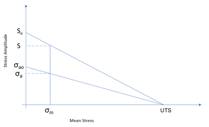
  1. Goodman or Soderberg
    (12) S F = s σ a = s e σ a 0 MathType@MTEF@5@5@+= feaagKart1ev2aaatCvAUfeBSjuyZL2yd9gzLbvyNv2CaerbuLwBLn hiov2DGi1BTfMBaeXatLxBI9gBaerbd9wDYLwzYbItLDharqqtubsr 4rNCHbGeaGqiVu0Je9sqqrpepC0xbbL8F4rqqrFfpeea0xe9Lq=Jc9 vqaqpepm0xbba9pwe9Q8fs0=yqaqpepae9pg0FirpepeKkFr0xfr=x fr=xb9adbaqaaeGaciGaaiaabeqaamaabaabaaGcbaGaam4uaiaadA eacqGH9aqpdaWcaaqaaiaadohaaeaacqaHdpWCdaWgaaWcbaGaamyy aaqabaaaaOGaeyypa0ZaaSaaaeaacaWGZbWaaSbaaSqaaiaadwgaae qaaaGcbaGaeq4Wdm3aaSbaaSqaaiaadggadaWgaaadbaGaaGimaaqa baaaleqaaaaaaaa@437B@

    s e MathType@MTEF@5@5@+= feaagKart1ev2aaatCvAUfeBSjuyZL2yd9gzLbvyNv2CaerbuLwBLn hiov2DGi1BTfMBaeXatLxBI9gBaerbd9wDYLwzYbItLDharqqtubsr 4rNCHbGeaGqiVu0Je9sqqrpepC0xbbL8F4rqqrFfpeea0xe9Lq=Jc9 vqaqpepm0xbba9pwe9Q8fs0=yqaqpepae9pg0FirpepeKkFr0xfr=x fr=xb9adbaqaaeGaciGaaiaabeqaamaabaabaaGcbaGaam4CamaaBa aaleaacaWGLbaabeaaaaa@3804@ = Target stress amplitude against the target life from the modified SN curve

    σ a 0 MathType@MTEF@5@5@+= feaagKart1ev2aaatCvAUfeBSjuyZL2yd9gzLbvyNv2CaerbuLwBLn hiov2DGi1BTfMBaeXatLxBI9gBaerbd9wDYLwzYbItLDharqqtubsr 4rNCHbGeaGqiVu0Je9sqqrpepC0xbbL8F4rqqrFfpeea0xe9Lq=Jc9 vqaqpepm0xbba9pwe9Q8fs0=yqaqpepae9pg0FirpepeKkFr0xfr=x fr=xb9adbaqaaeGaciGaaiaabeqaamaabaabaaGcbaGaeq4Wdm3aaS baaSqaaiaadggadaWgaaadbaGaaGimaaqabaaaleqaaaaa@39BD@ = Stress amplitude after mean stress correction


    Figure 12.
  2. Gerber
    (13) S F = s σ a = s e σ a 0 MathType@MTEF@5@5@+= feaagKart1ev2aaatCvAUfeBSjuyZL2yd9gzLbvyNv2CaerbuLwBLn hiov2DGi1BTfMBaeXatLxBI9gBaerbd9wDYLwzYbItLDharqqtubsr 4rNCHbGeaGqiVu0Je9sqqrpepC0xbbL8F4rqqrFfpeea0xe9Lq=Jc9 vqaqpepm0xbba9pwe9Q8fs0=yqaqpepae9pg0FirpepeKkFr0xfr=x fr=xb9adbaqaaeGaciGaaiaabeqaamaabaabaaGcbaGaam4uaiaadA eacqGH9aqpdaWcaaqaaiaadohaaeaacqaHdpWCdaWgaaWcbaGaamyy aaqabaaaaOGaeyypa0ZaaSaaaeaacaWGZbWaaSbaaSqaaiaadwgaae qaaaGcbaGaeq4Wdm3aaSbaaSqaaiaadggadaWgaaadbaGaaGimaaqa baaaleqaaaaaaaa@437B@


    Figure 13.
  3. Gerber2
    1. (14) σ m > 0 : S F = s σ a = s e σ a 0 MathType@MTEF@5@5@+= feaagKart1ev2aaatCvAUfeBSjuyZL2yd9gzLbvyNv2CaerbuLwBLn hiov2DGi1BTfMBaeXatLxBI9gBaerbd9wDYLwzYbItLDharqqtubsr 4rNCHbGeaGqiVu0Je9sqqrpepC0xbbL8F4rqqrFfpeea0xe9Lq=Jc9 vqaqpepm0xbba9pwe9Q8fs0=yqaqpepae9pg0FirpepeKkFr0xfr=x fr=xb9adbaqaaeGaciGaaiaabeqaamaabaabaaGceaqabeaacqaHdp WCdaWgaaWcbaGaamyBaaqabaGccqGH+aGpcaaIWaGaaiOoaaqaaiaa ykW7caaMc8Uaam4uaiaadAeacqGH9aqpdaWcaaqaaiaadohaaeaacq aHdpWCdaWgaaWcbaGaamyyaaqabaaaaOGaeyypa0ZaaSaaaeaacaWG ZbWaaSbaaSqaaiaadwgaaeqaaaGcbaGaeq4Wdm3aaSbaaSqaaiaadg gadaWgaaadbaGaaGimaaqabaaaleqaaaaaaaaa@4C03@
    2. (15) σ m 0 : S F = s σ a MathType@MTEF@5@5@+= feaagKart1ev2aaatCvAUfeBSjuyZL2yd9gzLbvyNv2CaerbuLwBLn hiov2DGi1BTfMBaeXatLxBI9gBaerbd9wDYLwzYbItLDharqqtubsr 4rNCHbGeaGqiVu0Je9sqqrpepC0xbbL8F4rqqrFfpeea0xe9Lq=Jc9 vqaqpepm0xbba9pwe9Q8fs0=yqaqpepae9pg0FirpepeKkFr0xfr=x fr=xb9adbaqaaeGaciGaaiaabeqaamaabaabaaGceaqabeaacqaHdp WCdaWgaaWcbaGaamyBaaqabaGccqGHKjYOcaaIWaGaaiOoaaqaaiaa ykW7caaMc8Uaam4uaiaadAeacqGH9aqpdaWcaaqaaiaadohaaeaacq aHdpWCdaWgaaWcbaGaamyyaaqabaaaaaaaaa@45B1@
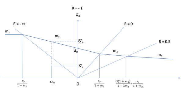
  4. FKM
    (16) S F = s ' e σ a MathType@MTEF@5@5@+= feaagKart1ev2aaatCvAUfeBSjuyZL2yd9gzLbvyNv2CaerbuLwBLn hiov2DGi1BTfMBaeXatLxBI9gBaerbd9wDYLwzYbItLDharqqtubsr 4rNCHbGeaGqiVu0Je9sqqrpepC0xbbL8F4rqqrFfpeea0xe9Lq=Jc9 vqaqpepm0xbba9pwe9Q8fs0=yqaqpepae9pg0FirpepeKkFr0xfr=x fr=xb9adbaqaaeGaciGaaiaabeqaamaabaabaaGcbaGaam4uaiaadA eacqGH9aqpdaWcaaqaaiaadohacaGGNaWaaSbaaSqaaiaadwgaaeqa aaGcbaGaeq4Wdm3aaSbaaSqaaiaadggaaeqaaaaaaaa@3E47@
    1. (17) σ m < s e 1 m 2 s ' e = m , ( σ m + s e 1 m 2 ) + s e 1 m 2 MathType@MTEF@5@5@+= feaagKart1ev2aaatCvAUfeBSjuyZL2yd9gzLbvyNv2CaerbuLwBLn hiov2DGi1BTfMBaeXatLxBI9gBaerbd9wDYLwzYbItLDharqqtubsr 4rNCHbGeaGqiVu0Je9sqqrpepC0xbbL8F4rqqrFfpeea0xe9Lq=Jc9 vqaqpepm0xbba9pwe9Q8fs0=yqaqpepae9pg0FirpepeKkFr0xfr=x fr=xb9adbaqaaeGaciGaaiaabeqaamaabaabaaGceaqabeaacqaHdp WCdaWgaaWcbaGaamyBaaqabaGccqGH8aapdaWcaaqaaiabgkHiTiaa dohadaWgaaWcbaGaamyzaaqabaaakeaacaaIXaGaeyOeI0IaamyBam aaBaaaleaacaaIYaaabeaaaaaakeaacaaMc8UaaGPaVlaaykW7caaM c8UaaGPaVlaaykW7caaMc8UaaGPaVlaaykW7caWGZbGaai4jamaaBa aaleaacaWGLbaabeaakiabg2da9iabgkHiTiaad2gacaGGSaGaaGPa VpaabmaabaGaeq4Wdm3aaSbaaSqaaiaad2gaaeqaaOGaey4kaSYaaS aaaeaacaWGZbWaaSbaaSqaaiaadwgaaeqaaaGcbaGaaGymaiabgkHi Tiaad2gadaWgaaWcbaGaaGOmaaqabaaaaaGccaGLOaGaayzkaaGaey 4kaSYaaSaaaeaacaWGZbWaaSbaaSqaaiaadwgaaeqaaaGcbaGaaGym aiabgkHiTiaad2gadaWgaaWcbaGaaGOmaaqabaaaaaaaaa@67E9@
    2. (18) s e 1 m 2 σ m < s e 1 + m 2 s ' e = m 2 σ m + s e MathType@MTEF@5@5@+= feaagKart1ev2aaatCvAUfeBSjuyZL2yd9gzLbvyNv2CaerbuLwBLn hiov2DGi1BTfMBaeXatLxBI9gBaerbd9wDYLwzYbItLDharqqtubsr 4rNCHbGeaGqiVu0Je9sqqrpepC0xbbL8F4rqqrFfpeea0xe9Lq=Jc9 vqaqpepm0xbba9pwe9Q8fs0=yqaqpepae9pg0FirpepeKkFr0xfr=x fr=xb9adbaqaaeGaciGaaiaabeqaamaabaabaaGceaqabeaadaWcaa qaaiabgkHiTiaadohadaWgaaWcbaGaamyzaaqabaaakeaacaaIXaGa eyOeI0IaamyBamaaBaaaleaacaaIYaaabeaaaaGccqGHKjYOcqaHdp WCdaWgaaWcbaGaamyBaaqabaGccqGH8aapdaWcaaqaaiaadohadaWg aaWcbaGaamyzaaqabaaakeaacaaIXaGaey4kaSIaamyBamaaBaaale aacaaIYaaabeaaaaaakeaacaaMc8UaaGPaVlaaykW7caaMc8UaaGPa VlaaykW7caaMc8UaaGPaVlaaykW7caaMc8UaaGPaVlaaykW7caaMc8 UaaGPaVlaaykW7caaMc8UaaGPaVlaaykW7caWGZbGaai4jamaaBaaa leaacaWGLbaabeaakiabg2da9iabgkHiTiaad2gadaWgaaWcbaGaaG OmaaqabaGccqaHdpWCdaWgaaWcbaGaamyBaaqabaGccqGHRaWkcaWG ZbWaaSbaaSqaaiaadwgaaeqaaaaaaa@7026@
    3. (19) s e 1 + m 2 σ m < 3 ( 1 + m 3 ) 1 + 3 m 3 · s e 1 + m 2 s ' e = m 3 ( σ m s e 1 + m 2 ) + s e 1 + m 2 MathType@MTEF@5@5@+= feaagKart1ev2aaatCvAUfeBSjuyZL2yd9gzLbvyNv2CaerbuLwBLn hiov2DGi1BTfMBaeXatLxBI9gBaerbd9wDYLwzYbItLDharqqtubsr 4rNCHbGeaGqiVu0Je9sqqrpepC0xbbL8F4rqqrFfpeea0xe9Lq=Jc9 vqaqpepm0xbba9pwe9Q8fs0=yqaqpepae9pg0FirpepeKkFr0xfr=x fr=xb9adbaqaaeGaciGaaiaabeqaamaabaabaaGceaqabeaadaWcaa qaaiaadohadaWgaaWcbaGaamyzaaqabaaakeaacaaIXaGaey4kaSIa amyBamaaBaaaleaacaaIYaaabeaaaaGccqGHKjYOcqaHdpWCdaWgaa WcbaGaamyBaaqabaGccqGH8aapdaWcaaqaaiaaiodacaGGOaGaaGym aiabgUcaRiaad2gadaWgaaWcbaGaaG4maaqabaGccaGGPaaabaGaaG ymaiabgUcaRiaaiodacaWGTbWaaSbaaSqaaiaaiodaaeqaaaaakiaa ykW7cqWIpM+zcaaMc8+aaSaaaeaacaWGZbWaaSbaaSqaaiaadwgaae qaaaGcbaGaaGymaiabgUcaRiaad2gadaWgaaWcbaGaaGOmaaqabaaa aaGcbaGaaGPaVlaaykW7caaMc8UaaGPaVlaaykW7caaMc8UaaGPaVl aaykW7caaMc8UaaGPaVlaaykW7caaMc8UaaGPaVlaaykW7caaMc8Ua aGPaVlaaykW7caaMc8Uaam4CaiaacEcadaWgaaWcbaGaamyzaaqaba GccqGH9aqpcqGHsislcaWGTbWaaSbaaSqaaiaaiodaaeqaaOWaaeWa aeaacqaHdpWCdaWgaaWcbaGaamyBaaqabaGccqGHsisldaWcaaqaai aadohadaWgaaWcbaGaamyzaaqabaaakeaacaaIXaGaey4kaSIaamyB amaaBaaaleaacaaIYaaabeaaaaaakiaawIcacaGLPaaacqGHRaWkda WcaaqaaiaadohadaWgaaWcbaGaamyzaaqabaaakeaacaaIXaGaey4k aSIaamyBamaaBaaaleaacaaIYaaabeaaaaaaaaa@8A4C@
    4. (20) 3 ( 1 + m 3 ) 1 + 3 m 3 · s e 1 + m 2 σ m s ' e = m 4 ( σ m 3 ( 1 + m 3 ) 1 + 3 m 3 · s e 1 + m 2 ) + 1 3 ( 3 ( 1 + m 2 ) 1 + 3 m 3 · s e 1 + m 2 ) MathType@MTEF@5@5@+= feaagKart1ev2aaatCvAUfeBSjuyZL2yd9gzLbvyNv2CaerbuLwBLn hiov2DGi1BTfMBaeXatLxBI9gBaerbd9wDYLwzYbItLDharqqtubsr 4rNCHbGeaGqiVu0Je9sqqrpepC0xbbL8F4rqqrFfpeea0xe9Lq=Jc9 vqaqpepm0xbba9pwe9Q8fs0=yqaqpepae9pg0FirpepeKkFr0xfr=x fr=xb9adbaqaaeGaciGaaiaabeqaamaabaabaaGceaqabeaadaWcaa qaaiaaiodacaGGOaGaaGymaiabgUcaRiaad2gadaWgaaWcbaGaaG4m aaqabaGccaGGPaaabaGaaGymaiabgUcaRiaaiodacaWGTbWaaSbaaS qaaiaaiodaaeqaaaaakiaaykW7cqWIpM+zcaaMc8+aaSaaaeaacaWG ZbWaaSbaaSqaaiaadwgaaeqaaaGcbaGaaGymaiabgUcaRiaad2gada WgaaWcbaGaaGOmaaqabaaaaOGaeyizImQaeq4Wdm3aaSbaaSqaaiaa d2gaaeqaaaGcbaGaaGPaVlaaykW7caaMc8UaaGPaVlaaykW7caaMc8 UaaGPaVlaaykW7caaMc8UaaGPaVlaaykW7caaMc8UaaGPaVlaaykW7 caaMc8UaaGPaVlaaykW7caaMc8Uaam4CaiaacEcadaWgaaWcbaGaam yzaaqabaGccqGH9aqpcqGHsislcaWGTbWaaSbaaSqaaiaaisdaaeqa aOWaaeWaaeaacqaHdpWCdaWgaaWcbaGaamyBaaqabaGccqGHsislda WcaaqaaiaaiodacaGGOaGaaGymaiabgUcaRiaad2gadaWgaaWcbaGa aG4maaqabaGccaGGPaaabaGaaGymaiabgUcaRiaaiodacaWGTbWaaS baaSqaaiaaiodaaeqaaaaakiaaykW7cqWIpM+zcaaMc8+aaSaaaeaa caWGZbWaaSbaaSqaaiaadwgaaeqaaaGcbaGaaGymaiabgUcaRiaad2 gadaWgaaWcbaGaaGOmaaqabaaaaaGccaGLOaGaayzkaaGaey4kaSYa aSaaaeaacaaIXaaabaGaaG4maaaadaqadaqaamaalaaabaGaaG4mai aacIcacaaIXaGaey4kaSIaamyBamaaBaaaleaacaaIYaaabeaakiaa cMcaaeaacaaIXaGaey4kaSIaaG4maiaad2gadaWgaaWcbaGaaG4maa qabaaaaOGaaGPaVlabl+y6NjaaykW7daWcaaqaaiaadohadaWgaaWc baGaamyzaaqabaaakeaacaaIXaGaey4kaSIaamyBamaaBaaaleaaca aIYaaabeaaaaaakiaawIcacaGLPaaaaaaa@A594@


    Figure 14.
  5. No Mean Stress Correction
    (21) S F = s e σ a MathType@MTEF@5@5@+= feaagKart1ev2aaatCvAUfeBSjuyZL2yd9gzLbvyNv2CaerbuLwBLn hiov2DGi1BTfMBaeXatLxBI9gBaerbd9wDYLwzYbItLDharqqtubsr 4rNCHbGeaGqiVu0Je9sqqrpepC0xbbL8F4rqqrFfpeea0xe9Lq=Jc9 vqaqpepm0xbba9pwe9Q8fs0=yqaqpepae9pg0FirpepeKkFr0xfr=x fr=xb9adbaqaaeGaciGaaiaabeqaamaabaabaaGcbaGaam4uaiaadA eacqGH9aqpdaWcaaqaaiaadohadaWgaaWcbaGaamyzaaqabaaakeaa cqaHdpWCdaWgaaWcbaGaamyyaaqabaaaaaaa@3D9C@
Stress Ratio = Constant
  1. Goodman
    (22) S F = O B O A = 1 ( σ a s e + σ m U T S ) MathType@MTEF@5@5@+= feaagKart1ev2aaatCvAUfeBSjuyZL2yd9gzLbvyNv2CaerbuLwBLn hiov2DGi1BTfMBaeXatLxBI9gBaerbd9wDYLwzYbItLDharqqtubsr 4rNCHbGeaGqiVu0Je9sqqrpepC0xbbL8F4rqqrFfpeea0xe9Lq=Jc9 vqaqpepm0xbba9pwe9Q8fs0=yqaqpepae9pg0FirpepeKkFr0xfr=x fr=xb9adbaqaaeGaciGaaiaabeqaamaabaabaaGcbaGaam4uaiaadA eacqGH9aqpdaWcaaqaaiaad+eacaWGcbaabaGaam4taiaadgeaaaGa eyypa0ZaaSaaaeaacaaIXaaabaWaaeWaaeaadaWcaaqaaiabeo8aZn aaBaaaleaacaWGHbaabeaaaOqaaiaadohadaWgaaWcbaGaamyzaaqa baaaaOGaey4kaSYaaSaaaeaacqaHdpWCdaWgaaWcbaGaamyBaaqaba aakeaacaWGvbGaamivaiaadofaaaaacaGLOaGaayzkaaaaaaaa@4AAD@


    Figure 15.
  2. Gerber
    1. (23) If σ m =0: SF= s e σ a MathType@MTEF@5@5@+= feaagKart1ev2aaatCvAUfeBSjuyZL2yd9gzLbvyNv2CaerbuLwBLn hiov2DGi1BTfMBaeXatLxBI9gBaerbd9wDYLwzYbItLDharqqtubsr 4rNCHbGeaGqiVu0Je9sqqrpepC0xbbL8F4rqqrFfpeea0xe9Lq=Jc9 vqaqpepm0xbba9pwe9Q8fs0=yqaqpepae9pg0FirpepeKkFr0xfr=x fr=xb9adbaqaaeGaciGaaiaabeqaamaabaabaaGceaqabeaacaqGjb GaaeOzaiaaykW7cqaHdpWCdaWgaaWcbaGaamyBaaqabaGccqGH9aqp caaIWaGaaiOoaaqaaiaaykW7caaMc8UaaGPaVlaaykW7caaMc8UaaG PaVlaaykW7caaMc8UaaGPaVlaaykW7caaMc8UaaGPaVlaaykW7caaM c8UaaGPaVlaaykW7caWGtbGaamOraiabg2da9maalaaabaGaam4Cam aaBaaaleaacaWGLbaabeaaaOqaaiabeo8aZnaaBaaaleaacaWGHbaa beaaaaaaaaa@5EFC@
    2. (24) If σ m 0: SF= 1 2 ( UTS σ m ) 2 · σ a s e [ 1+ 1+ ( 2 s e σ m UTS σ a ) 2 ] MathType@MTEF@5@5@+= feaagKart1ev2aaatCvAUfeBSjuyZL2yd9gzLbvyNv2CaerbuLwBLn hiov2DGi1BTfMBaeXatLxBI9gBaerbd9wDYLwzYbItLDharqqtubsr 4rNCHbGeaGqiVu0Je9sqqrpepC0xbbL8F4rqqrFfpeea0xe9Lq=Jc9 vqaqpepm0xbba9pwe9Q8fs0=yqaqpepae9pg0FirpepeKkFr0xfr=x fr=xb9adbaqaaeGaciGaaiaabeqaamaabaabaaGceaqabeaacaqGjb GaaeOzaiaaykW7cqaHdpWCdaWgaaWcbaGaamyBaaqabaGccqGHGjsU caaIWaGaaiOoaaqaaiaaykW7caaMc8UaaGPaVlaaykW7caaMc8UaaG PaVlaaykW7caaMc8UaaGPaVlaaykW7caaMc8UaaGPaVlaaykW7caaM c8UaaGPaVlaaykW7caWGtbGaamOraiabg2da9maalaaabaGaaGymaa qaaiaaikdaaaWaaeWaaeaadaWcaaqaaiaadwfacaWGubGaam4uaaqa aiabeo8aZnaaBaaaleaacaWGTbaabeaaaaaakiaawIcacaGLPaaada ahaaWcbeqaaiaaikdaaaGccaaMc8UaeS4JPFMaaGPaVpaalaaabaGa eq4Wdm3aaSbaaSqaaiaadggaaeqaaaGcbaGaam4CamaaBaaaleaaca WGLbaabeaaaaGcdaWadaqaaiabgkHiTiaaigdacqGHRaWkdaGcaaqa aiaaigdacqGHRaWkdaqadaqaamaalaaabaGaaGOmaiaadohadaWgaa WcbaGaamyzaaqabaGccqaHdpWCdaWgaaWcbaGaamyBaaqabaaakeaa caWGvbGaamivaiaadofacaaMc8UaeyyXICTaaGPaVlabeo8aZnaaBa aaleaacaWGHbaabeaaaaaakiaawIcacaGLPaaadaahaaWcbeqaaiaa ikdaaaaabeaaaOGaay5waiaaw2faaaaaaa@8814@
  3. Gerber2
    1. (25) If  σ m 0: SF= s e σ a MathType@MTEF@5@5@+= feaagKart1ev2aaatCvAUfeBSjuyZL2yd9gzLbvyNv2CaerbuLwBLn hiov2DGi1BTfMBaeXatLxBI9gBaerbd9wDYLwzYbItLDharqqtubsr 4rNCHbGeaGqiVu0Je9sqqrpepC0xbbL8F4rqqrFfpeea0xe9Lq=Jc9 vqaqpepm0xbba9pwe9Q8fs0=yqaqpepae9pg0FirpepeKkFr0xfr=x fr=xb9adbaqaaeGaciGaaiaabeqaamaabaabaaGceaqabeaacaqGjb GaaeOzaiaabccacqaHdpWCdaWgaaWcbaGaamyBaaqabaGccqGHKjYO caaIWaGaaiOoaaqaaiaaysW7caaMe8UaaGjbVlaaysW7caaMe8UaaG jbVlaaysW7caaMe8UaaGjbVlaaysW7caaMe8Uaam4uaiaadAeacqGH 9aqpdaWcaaqaaiaadohadaWgaaWcbaGaamyzaaqabaaakeaacqaHdp WCdaWgaaWcbaGaamyyaaqabaaaaaaaaa@5722@
    2. (26) If σ m 0: SF= 1 2 ( UTS σ m ) 2 · σ a s e [ 1+ 1+ ( 2 s e σ m UTS σ a ) 2 ] MathType@MTEF@5@5@+= feaagKart1ev2aaatCvAUfeBSjuyZL2yd9gzLbvyNv2CaerbuLwBLn hiov2DGi1BTfMBaeXatLxBI9gBaerbd9wDYLwzYbItLDharqqtubsr 4rNCHbGeaGqiVu0Je9sqqrpepC0xbbL8F4rqqrFfpeea0xe9Lq=Jc9 vqaqpepm0xbba9pwe9Q8fs0=yqaqpepae9pg0FirpepeKkFr0xfr=x fr=xb9adbaqaaeGaciGaaiaabeqaamaabaabaaGceaqabeaacaqGjb GaaeOzaiaaykW7cqaHdpWCdaWgaaWcbaGaamyBaaqabaGccqGHLjYS caaIWaGaaiOoaaqaaiaaykW7caaMc8UaaGPaVlaaykW7caaMc8UaaG PaVlaaykW7caaMc8UaaGPaVlaaykW7caaMc8UaaGPaVlaaykW7caaM c8UaaGPaVlaaykW7caWGtbGaamOraiabg2da9maalaaabaGaaGymaa qaaiaaikdaaaWaaeWaaeaadaWcaaqaaiaadwfacaWGubGaam4uaaqa aiabeo8aZnaaBaaaleaacaWGTbaabeaaaaaakiaawIcacaGLPaaada ahaaWcbeqaaiaaikdaaaGccaaMc8UaeS4JPFMaaGPaVpaalaaabaGa eq4Wdm3aaSbaaSqaaiaadggaaeqaaaGcbaGaam4CamaaBaaaleaaca WGLbaabeaaaaGcdaWadaqaaiabgkHiTiaaigdacqGHRaWkdaGcaaqa aiaaigdacqGHRaWkdaqadaqaamaalaaabaGaaGOmaiaadohadaWgaa WcbaGaamyzaaqabaGccqaHdpWCdaWgaaWcbaGaamyBaaqabaaakeaa caWGvbGaamivaiaadofacaaMc8UaeyyXICTaaGPaVlabeo8aZnaaBa aaleaacaWGHbaabeaaaaaakiaawIcacaGLPaaadaahaaWcbeqaaiaa ikdaaaaabeaaaOGaay5waiaaw2faaaaaaa@8813@
  4. FKM
    (27) S F = s e σ a 0 MathType@MTEF@5@5@+= feaagKart1ev2aaatCvAUfeBSjuyZL2yd9gzLbvyNv2CaerbuLwBLn hiov2DGi1BTfMBaeXatLxBI9gBaerbd9wDYLwzYbItLDharqqtubsr 4rNCHbGeaGqiVu0Je9sqqrpepC0xbbL8F4rqqrFfpeea0xe9Lq=Jc9 vqaqpepm0xbba9pwe9Q8fs0=yqaqpepae9pg0FirpepeKkFr0xfr=x fr=xb9adbaqaaeGaciGaaiaabeqaamaabaabaaGcbaGaam4uaiaadA eacqGH9aqpdaWcaaqaaiaadohadaWgaaWcbaGaamyzaaqabaaakeaa cqaHdpWCdaWgaaWcbaGaamyyamaaBaaameaacaaIWaaabeaaaSqaba aaaaaa@3E8E@

    σ a 0 MathType@MTEF@5@5@+= feaagKart1ev2aaatCvAUfeBSjuyZL2yd9gzLbvyNv2CaerbuLwBLn hiov2DGi1BTfMBaeXatLxBI9gBaerbd9wDYLwzYbItLDharqqtubsr 4rNCHbGeaGqiVu0Je9sqqrpepC0xbbL8F4rqqrFfpeea0xe9Lq=Jc9 vqaqpepm0xbba9pwe9Q8fs0=yqaqpepae9pg0FirpepeKkFr0xfr=x fr=xb9adbaqaaeGaciGaaiaabeqaamaabaabaaGcbaGaeq4Wdm3aaS baaSqaaiaadggadaWgaaadbaGaaGimaaqabaaaleqaaaaa@39BD@ = Corrected Stress Amplitude in Constant R mean stress correction

  5. No Mean Stress Correction
    (28) SF= s e s a MathType@MTEF@5@5@+= feaagKart1ev2aaatCvAUfeBSjuyZL2yd9gzLbvyNv2CaerbuLwBLn hiov2DGi1BTfMBaeXatLxBI9gBaerbd9wDYLwzYbItLDharqqtubsr 4rNCHbGeaGqiVu0Je9sqqrpepC0xbbL8F4rqqrFfpeea0xe9Lq=Jc9 vqaqpepm0xbba9pwe9Q8fs0=yqaqpepae9pg0FirpepeKkFr0xfr=x fr=xb9adbaqaaeGaciGaaiaabeqaamaabaabaaGcbaGaam4uaiaadA eacqGH9aqpdaWcaaqaaiaadohadaWgaaWcbaGaamyzaaqabaaakeaa caWGZbWaaSbaaSqaaiaadggaaeqaaaaaaaa@3CD1@

Strain-Life (E-N) Approach

Strain-life analysis is based on the fact that many critical locations such as notch roots have stress concentration, which will have obvious plastic deformation during the cyclic loading before fatigue failure. Thus, the elastic-plastic strain results are essential for performing strain-life analysis.

Neuber Correction

Neuber correction is the most popular practice to correct elastic analysis results into elastic-plastic results.

In order to derive the local stress from the nominal stress that is easier to obtain, the concentration factors are introduced such as the local stress concentration factor K σ , and the local strain concentration factor K ε .(29) K σ = σ / S (30) K ε = ε / e
Where, σ is the local stress, ε is the local strain, S is the nominal stress, and e is the nominal strain. If nominal stress and local stress are both elastic, the local stress concentration factor is equal to the local strain concentration factor. However, if the plastic strain is present, the relationship between K σ and K ε no long holds. Thereafter, focusing on this situation, Neuber introduced a theoretically elastic stress concentration factor K t defined as:(31) K t 2 = K σ K ε
Substitute Equation 29 and Equation 30 into Equation 31, the theoretical stress concentration factor K t can be rewritten as:(32) K t 2 =( σ S )( ε e )
Through linear static FEA, the local stress instead of nominal stress is provided, which implies the effect of the geometry in Equation 32 is removed, thus you can set K t as 1 and rewrite Equation 32 as:(33) σε= σ e ε e

Where, σ e , ε e is locally elastic stress and locally elastic strain obtained from elastic analysis, σ , ε the stress and strain at the presence of plastic strain. Both σ and ε can be calculated from Equation 33 together with the equations for the cyclic stress-strain curve and hysteresis loop.

Monotonic Stress-Strain Behavior

Relative to the current configuration, the true stress and strain relationship can be defined as:(34) σ = P / A (35) ε = l l d l l = ln ( 1 + l l 0 l 0 )

Where, A is the current cross-section area, l is the current objects length, l 0 is the initial objects length, and σ and ε are the true stress and strain, respectively, Figure 16 shows the monotonic stress-strain curve in true stress-strain space. In the whole process, the stress continues increasing to a large value until the object fails at C.


Figure 16. Monotonic Stress-Strain Curve
The curve in Figure 16 is comprised of two typical segments, namely the elastic segment OA and plastic segment AC. The segment OA keeps the linear relationship between stress and elastic strain following Hooke Law:(36) σ=E ε e
Where, E is elastic modulus and ε e is elastic strain. The formula can also be rewritten as:(37) ε e =σ/E
by expressing elastic strain in terms of stress. For most of materials, the relationship between the plastic strain and the stress can be represented by a simple power law of the form:(38) σ=K ( ε p ) n
Where, ε p is plastic strain, K is strength coefficient, and n is work hardening coefficient. Similarly, the plastic strain can be expressed in terms of stress as:(39) ε p = ( σ K ) 1/n
The total strain induced by loading the object up to point B or D is the sum of plastic strain and elastic strain:(40) ε= ε e + ε p = σ E + ( σ K ' ) 1/ n ' MathType@MTEF@5@5@+= feaagKart1ev2aaatCvAUfeBSjuyZL2yd9gzLbvyNv2CaerbuLwBLn hiov2DGi1BTfMBaeXatLxBI9gBaerbd9wDYLwzYbItLDharqqtubsr 4rNCHbGeaGqiVu0Je9sqqrpepC0xbbL8F4rqqrFfpeea0xe9Lq=Jc9 vqaqpepm0xbba9pwe9Q8fs0=yqaqpepae9pg0FirpepeKkFr0xfr=x fr=xb9adbaqaaeGaciGaaiaabeqaamaabaabaaGcbaGaeqyTduMaey ypa0JaeqyTdu2aaSbaaSqaaiaadwgaaeqaaOGaey4kaSIaeqyTdu2a aSbaaSqaaiaadchaaeqaaOGaeyypa0ZaaSaaaeaacqaHdpWCaeaaca WGfbaaaiabgUcaRmaabmaabaWaaSaaaeaacqaHdpWCaeaacaWGlbWa aWbaaSqabeaacaGGNaaaaaaaaOGaayjkaiaawMcaamaaCaaaleqaba GaaGymaiaac+cacaWGUbWaaWbaaWqabeaacaGGNaaaaaaaaaa@4C18@

Cyclic Stress-Strain Curve

Material exhibits different behavior under cyclic load compared with that of monotonic load. Generally, there are four kinds of response.
  • Stable state
  • Cyclically hardening
  • Cyclically softening
  • Softening or hardening depending on strain range
Which response will occur depends on its nature and initial condition of heat treatment. Figure 17 illustrates the effect of cyclic hardening and cyclic softening where the first two hysteresis loops of two different materials are plotted. In both cases, the strain is constrained to change in fixed range, while the stress is allowed to change arbitrarily. If the stress range increases relative to the former cycle under fixed strain range, as shown in the upper portion of Figure 17, it is called cyclic hardening; otherwise, it is called cyclic softening, as shown in the lower portion of Figure 17. Cyclic response of material can also be described by specifying the stress range and leaving strain unconstrained. If the strain range increases relative to the former cycle under fixed stress range, it is called cyclic softening; otherwise, it is called cyclic hardening. In fact, the cyclic behavior of material will reach a steady state after a short time which generally occupies less than 10 percent of the material total life. Through specifying different strain ranges, a series of hysteresis loops at steady state can be obtained. By placing these hysteresis loops in one coordinate system, as shown in Figure 18, the line connecting all the vertices of these hysteresis loops determine cyclic stress-strain curve which can be expressed in the similar form with monotonic stress-strain curve as:


Figure 17. Material Cyclic Response


Figure 18. Definition of Stable Stress-Strain Curve
(41) ε= ε e + ε p = σ E + ( σ K ' ) 1/ n ' MathType@MTEF@5@5@+= feaagKart1ev2aaatCvAUfeBSjuyZL2yd9gzLbvyNv2CaerbuLwBLn hiov2DGi1BTfMBaeXatLxBI9gBaerbd9wDYLwzYbItLDharqqtubsr 4rNCHbGeaGqiVu0Je9sqqrpepC0xbbL8F4rqqrFfpeea0xe9Lq=Jc9 vqaqpepm0xbba9pwe9Q8fs0=yqaqpepae9pg0FirpepeKkFr0xfr=x fr=xb9adbaqaaeGaciGaaiaabeqaamaabaabaaGcbaGaeqyTduMaey ypa0JaeqyTdu2aaSbaaSqaaiaadwgaaeqaaOGaey4kaSIaeqyTdu2a aSbaaSqaaiaadchaaeqaaOGaeyypa0ZaaSaaaeaacqaHdpWCaeaaca WGfbaaaiabgUcaRmaabmaabaWaaSaaaeaacqaHdpWCaeaacaWGlbWa aWbaaSqabeaacaGGNaaaaaaaaOGaayjkaiaawMcaamaaCaaaleqaba GaaGymaiaac+cacaWGUbWaaWbaaWqabeaacaGGNaaaaaaaaaa@4C18@
Where,
K ' MathType@MTEF@5@5@+= feaagKart1ev2aaatCvAUfeBSjuyZL2yd9gzLbvyNv2CaerbuLwBLn hiov2DGi1BTfMBaeXatLxBI9gBaerbd9wDYLwzYbItLDharqqtubsr 4rNCHbGeaGqiVu0Je9sqqrpepC0xbbL8F4rqqrFfpeea0xe9Lq=Jc9 vqaqpepm0xbba9pwe9Q8fs0=yqaqpepae9pg0FirpepeKkFr0xfr=x fr=xb9adbaqaaeGaciGaaiaabeqaamaabaabaaGcbaGaam4samaaCa aaleqabaGaai4jaaaaaaa@379E@
Cyclic strength coefficient
n ' MathType@MTEF@5@5@+= feaagKart1ev2aaatCvAUfeBSjuyZL2yd9gzLbvyNv2CaerbuLwBLn hiov2DGi1BTfMBaeXatLxBI9gBaerbd9wDYLwzYbItLDharqqtubsr 4rNCHbGeaGqiVu0Je9sqqrpepC0xbbL8F4rqqrFfpeea0xe9Lq=Jc9 vqaqpepm0xbba9pwe9Q8fs0=yqaqpepae9pg0FirpepeKkFr0xfr=x fr=xb9adbaqaaeGaciGaaiaabeqaamaabaabaaWcbaGaamOBamaaCa aameqabaGaai4jaaaaaaa@37C3@
Strain cyclic hardening exponent

Hysteresis Loop Shape

Bauschinger observed that after the initial load had caused plastic strain, load reversal caused materials to exhibit anisotropic behavior. Based on experiment evidence, Massing put forward the hypothesis that a stress-strain hysteresis loop is geometrically similar to the cyclic stress strain curve, but with twice the magnitude. This implies that when the quantity ( Δ ε , Δ σ ) is two times of ( ε , σ ), the stress-strain cycle will lie on the hysteresis loop. This can be expressed with formulas:(42) Δ σ = 2 σ (43) Δ ε = 2 ε
Expressing σ in terms of Δσ, ε in terms of Δε, and substituting it into Equation 41, the hysteresis loop formula can be calculated as:(44) Δε= Δσ E +2 ( Δσ 2K' ) 1/n'
Almost a century ago, Basquin observed the linear relationship between stress and fatigue life in log scale when the stress is limited. He put forward the following fatigue formula controlled by stress:(45) σ a = σ ' f ( 2 N f ) b
Where, σ a is the stress amplitude, σ f ' is the fatigue strength coefficient, and b is the fatigue strength exponent. Later in the 1950s, Coffin and Manson independently proposed that plastic strain may also be related with fatigue life by a simple power law:(46) ε a p = ε ' f ( 2 N f ) c
Where, ε a p is the plastic strain amplitude, ε ' f is the fatigue ductility coefficient, and c is the fatigue ductility exponent. Morrow combined the work of Basquin, Coffin and Manson to consider both elastic strain and plastic strain contribution to the fatigue life. He found out that the total strain has more direct correlation with fatigue life. By applying Hooke Law, Basquin rule can be rewritten as:(47) ε a e = σ a E = σ ' f E ( 2 N f ) b
Where, ε a e is elastic strain amplitude. Total strain amplitude, which is the sum of the elastic strain and plastic stain, therefore, can be described by applying Basquin formula and Coffin-Manson formula:(48) ε a = ε a e + ε a p = σ ' f E ( 2 N f ) b + ε ' f ( 2 N f ) c
Where, ε a is the total strain amplitude, the other variable is the same with above.


Figure 19. Strain-Life Curve in Log Scale

Mean Stress Correction

The fatigue experiments carried out in the laboratory are always fully reversed, whereas in practice, the mean stress is inevitable, thus the fatigue law established by the fully reversed experiments must be corrected before applied to engineering problems.

Morrow:
Morrow is the first to consider the effect of mean stress through introducing the mean stress σ 0 in fatigue strength coefficient by:(49) ε a e = ( σ ' f σ 0 ) E ( 2 N f ) b
Thus, the entire fatigue life formula becomes:(50) ε a = ( σ ' f σ 0 ) E ( 2 N f ) b + ε f ' ( 2 N f ) c MathType@MTEF@5@5@+= feaagKart1ev2aqatCvAUfeBSjuyZL2yd9gzLbvyNv2CaerbuLwBLn hiov2DGi1BTfMBaeXatLxBI9gBaerbd9wDYLwzYbItLDharqqtubsr 4rNCHbGeaGqiVu0Je9sqqrpepC0xbbL8F4rqqrFfpeea0xe9Lq=Jc9 vqaqpepm0xbba9pwe9Q8fs0=yqaqpepae9pg0FirpepeKkFr0xfr=x fr=xb9adbaqaaeGaciGaaiaabeqaamaabaabaaGcbaGaeqyTdu2aa0 baaSqaaiaadggaaeaacaWGLbaaaOGaeyypa0ZaaSaaaeaadaqadaqa aiabeo8aZjaacEcadaWgaaWcbaGaamOzaaqabaGccqGHsislcqaHdp WCdaWgaaWcbaGaaGimaaqabaaakiaawIcacaGLPaaaaeaacaWGfbaa amaabmaabaGaaGOmaiaad6eadaWgaaWcbaGaamOzaaqabaaakiaawI cacaGLPaaadaahaaWcbeqaaiaadkgaaaGccqGHRaWkcqaH1oqzdaqh aaWcbaGaamOzaaqaaiaacEcaaaGcdaqadaqaaiaaikdacaWGobWaaS baaSqaaiaadAgaaeqaaaGccaGLOaGaayzkaaWaaWbaaSqabeaacaWG Jbaaaaaa@5338@

Morrow's equation is consistent with the observation that mean stress effects are significant at low value of plastic strain and of little effect at high plastic strain.

MORROW2:

Improves the MORROW method by ignoring the effect of negative mean stress.

Smith, Watson and Topper:
Smith, Watson and Topper proposed a different method to account for the effect of mean stress by considering the maximum stress during one cycle (for convenience, this method is called SWT in the following). In this case, the damage parameter is modified as the product of the maximum stress and strain amplitude in one cycle.(51) ε a S W T σ max = ε a σ a = σ a ( σ ' f E ( 2 N f ) b + ε ' f ( 2 N f ) c ) MathType@MTEF@5@5@+= feaagKart1ev2aqatCvAUfeBSjuyZL2yd9gzLbvyNv2CaerbuLwBLn hiov2DGi1BTfMBaeXatLxBI9gBaerbd9wDYLwzYbItLDharqqtubsr 4rNCHbGeaGqiVu0Je9sqqrpepC0xbbL8F4rqqrFfpeea0xe9Lq=Jc9 vqaqpepm0xbba9pwe9Q8fs0=yqaqpepae9pg0FirpepeKkFr0xfr=x fr=xb9adbaqaaeGaciGaaiaabeqaamaabaabaaGcbaGaeqyTdu2aa0 baaSqaaiaadggaaeaacaWGtbGaam4vaiaadsfaaaGccqaHdpWCdaWg aaWcbaGaciyBaiaacggacaGG4baabeaakiabg2da9iabew7aLnaaBa aaleaacaWGHbaabeaakiabeo8aZnaaBaaaleaacaWGHbaabeaakiab g2da9iabeo8aZnaaBaaaleaacaWGHbaabeaakmaabmaabaWaaSaaae aacqaHdpWCcaGGNaWaaSbaaSqaaiaadAgaaeqaaaGcbaGaamyraaaa daqadaqaaiaaikdacaWGobWaaSbaaSqaaiaadAgaaeqaaaGccaGLOa GaayzkaaWaaWbaaSqabeaacaWGIbaaaOGaey4kaSIaeqyTduMaai4j amaaBaaaleaacaWGMbaabeaakmaabmaabaGaaGOmaiaad6eadaWgaa WcbaGaamOzaaqabaaakiaawIcacaGLPaaadaahaaWcbeqaaiaadoga aaaakiaawIcacaGLPaaaaaa@5F98@

The SWT method will predict that no damage will occur when the maximum stress is zero or negative, which is not consistent with the reality.

When comparing the two methods, the SWT method predicted conservative life for loads predominantly tensile, whereas, the Morrow approach provides more realistic results when the load is predominantly compressive.

Damage Accumulation Model

In the E-N approach, use the same damage accumulation model as the S-N approach, which is Palmgren-Miner's linear damage summation rule.