HL-T: 1060 Seam Weld (Fillet)
In this tutorial you will:
- Import a model to HyperLife
- Select the Weld module and define its required parameters
- Create materials and assign them to the welds and sheet groups
- Assign load histories for scaling the stresses from FEA subcases
- Evaluate and view results
Before you begin, copy the file(s) used in this tutorial to your
working directory.
- HL-1060\Seam-Fillet.h3d
- HL-1060\Seam-Fillet.gpf
- Load_History_Files\load1.csv
- Load_History_Files\load2.csv
Import the Model
Note: Only OptiStruct and Nastran results are supported.
-
From the Home tools, Files tool group, click the Open Model tool.

Figure 1. -
Click Apply.
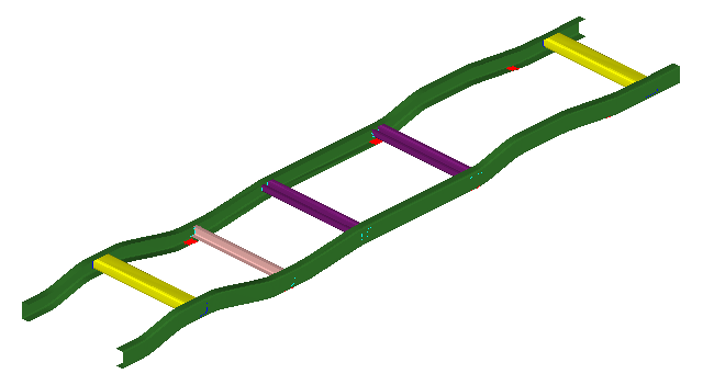
Figure 2.
Tip: Quickly import the model by dragging and
dropping the .h3d file from
a windows browser into the HyperLife
modeling window.
Define the Fatigue Module
-
From the Setup tools, click the arrow next to the
fatigue module icon and select the Weld tool from the
list of options.

Figure 3.The Weld dialog opens. -
Accept all other default parameters.
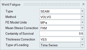
Figure 4.
Assign Materials
-
From the Setup tools, click the
Material tool.

Figure 5.The Assign Material dialog opens. -
Create a bending material.
-
Click
 to create a new material.
-
Accept all other default settings then click Plot &
Save.
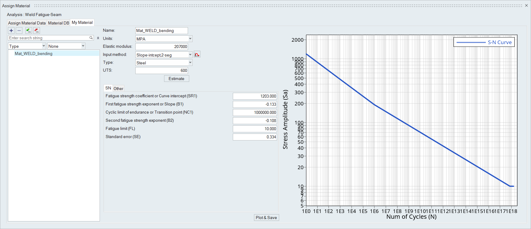
Figure 6.
-
Click
-
Create a membrane material.
-
Staying in the My Material tab, click to create another material.
-
Accept all other default settings then click Plot &
Save.
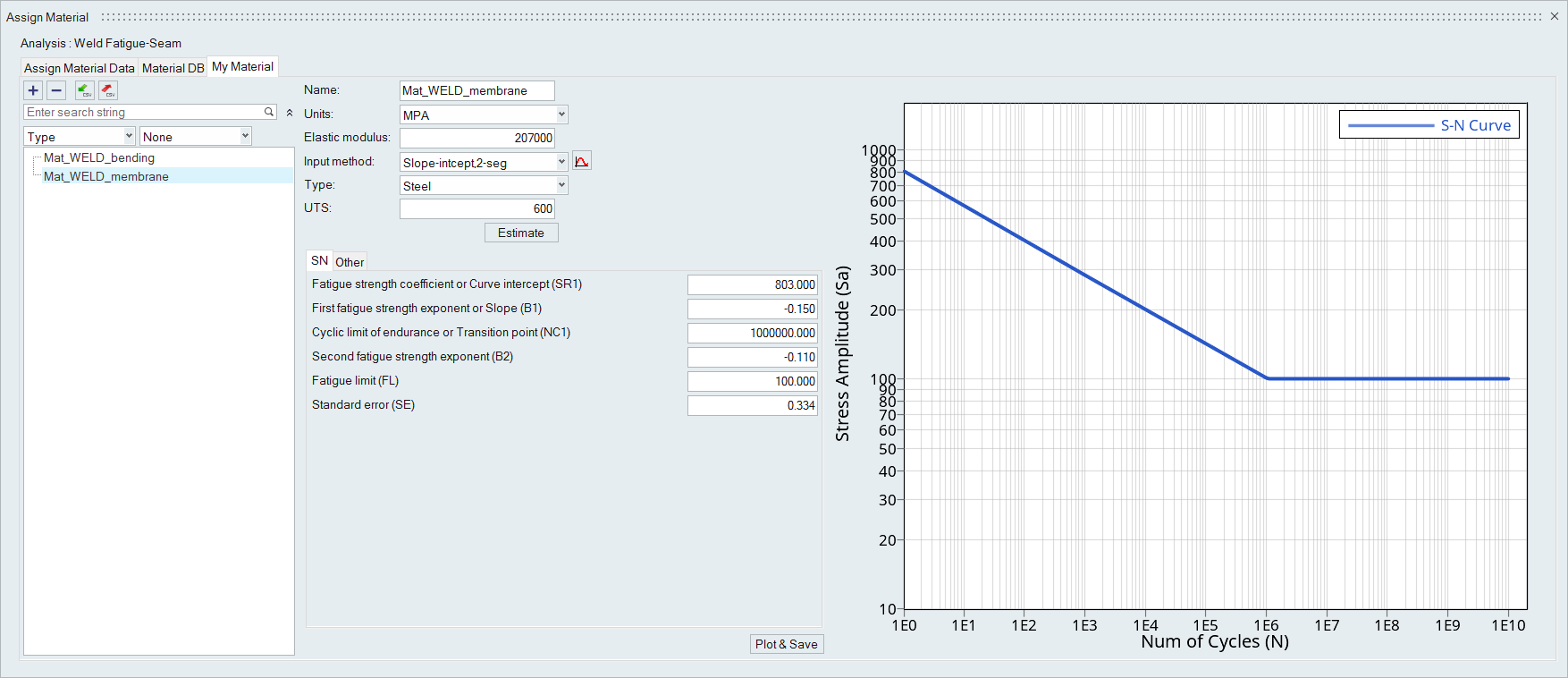
Figure 7.
-
Staying in the My Material tab, click
-
Set TREF_N to 0.1 for both components.
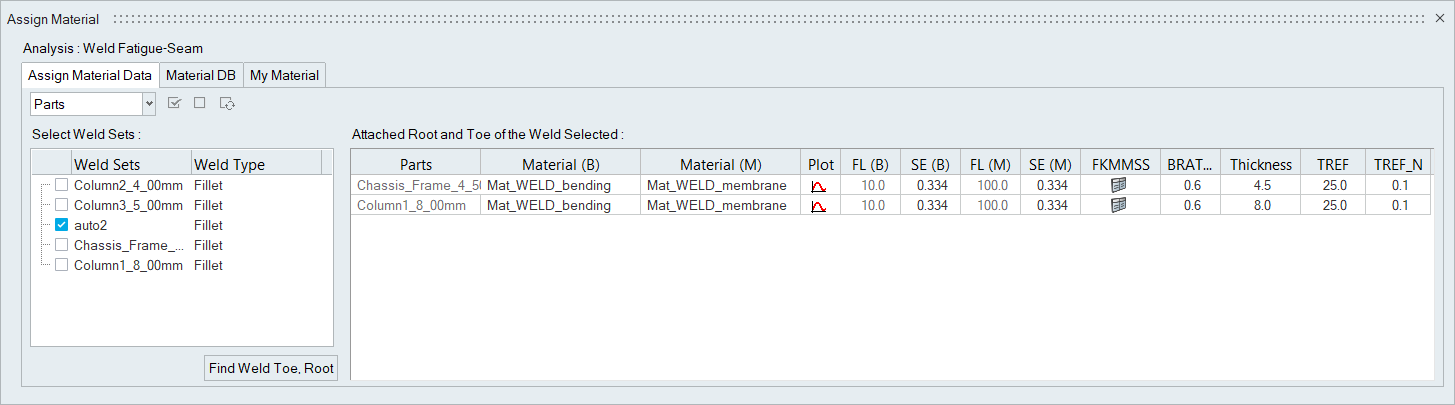
Figure 8.
Assign Load Histories
-
From the Setup tools, click the
Load Map tool.

Figure 9.The Load Map dialog opens. -
Click
 in the Choose File
field and browse for load1.csv.
in the Choose File
field and browse for load1.csv.
-
Click to add the load case.
- Optional:
Click
 to view a plot of the loads.
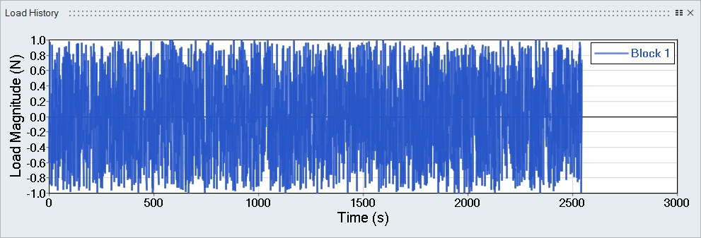
Figure 10. Load 1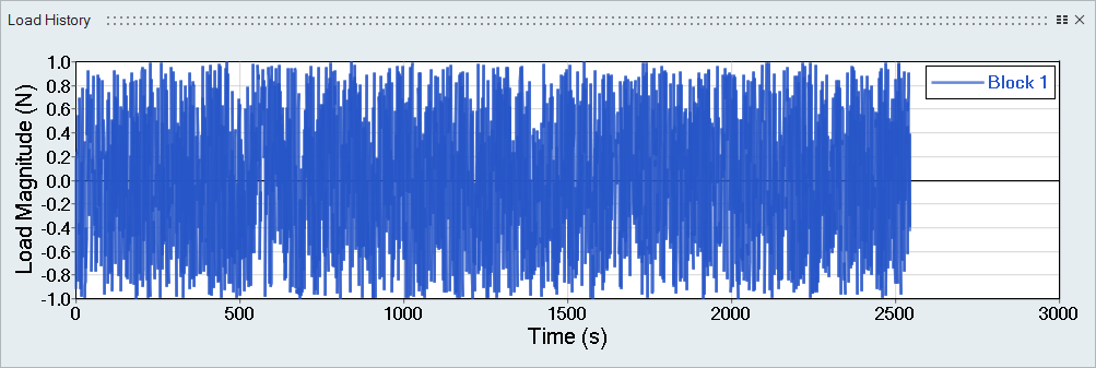
Figure 11. Load 2Tip: Expand the width of the dialog to view a clearer picture of the plot. -
Select both the Block 1 channel under load1 and
Subcase 1, then click to create the first event.
-
Next, select both Block 1 channels, Subcase
2, and Subcase 3 then click .
A second event is created.Tip: Hold Control while left-clicking to select multiple options.
-
Similarly, set the Scale to 0.6 for all three
subcases.
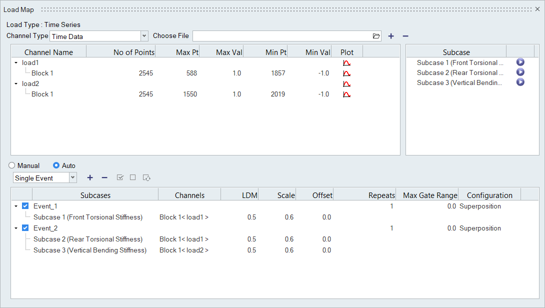
Figure 12.
Evaluate and View Results
-
From the Evaluate tool group, click the Run Analysis tool.

Figure 13.The Evaluate dialog opens.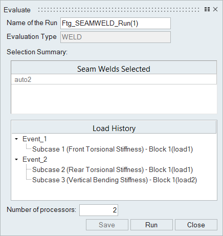
Figure 14. -
Use the Results Explorer to
visualize various types of results.
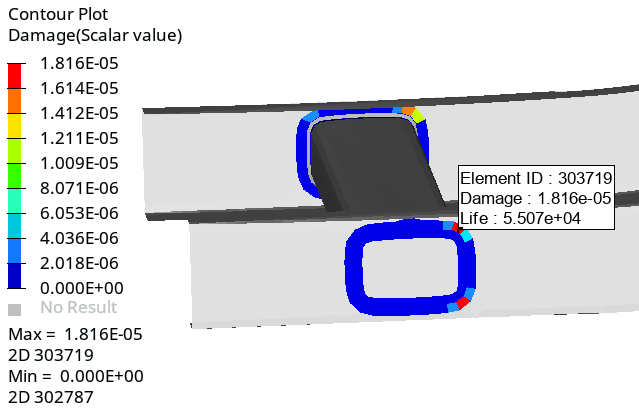
Figure 15.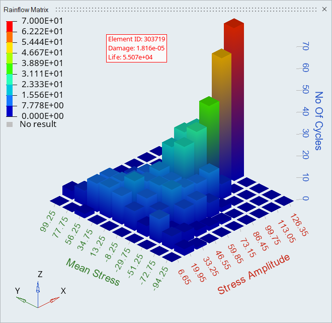
Figure 16.The life expectancy for the worst element is 5.607e4 cycles.