HL-T: 1100 Stress Life (S-N) Using Stress History Created from Modal Participation Factors (via a *.pch file) and Modal Stress

In this tutorial you will:
  • Import a model to HyperLife
  • Select the SN module with a Modal Superposition loading type and define its required parameters
  • Create and assign a material
  • Assign a *.pch file (containing modal participation factors) to modal stresses
  • Evaluate and view results
Before you begin, copy the file(s) used in this tutorial to your working directory.
  • HL-1100\Rear_Truss.h3d
  • Rear_Truss_modal.pch
Note: The aim of this tutorial is to:
  1. Create stress history from modal participation factors and modal stresses.
    For the complete time interval, stress history is given by: σ i j ( t ) = k P k ( t ) * σ i j , k MathType@MTEF@5@5@+= feaagKart1ev2aaatCvAUfeBSjuyZL2yd9gzLbvyNv2CaerbuLwBLn hiov2DGi1BTfMBaeXatLxBI9gBaerbd9wDYLwzYbItLDharqqtubsr 4rNCHbGeaGqiVu0Je9sqqrpepC0xbbL8F4rqqrFfpeea0xe9Lq=Jc9 vqaqpepm0xbba9pwe9Q8fs0=yqaqpepae9pg0FirpepeKkFr0xfr=x fr=xb9adbaqaaeGaciGaaiaabeqaamaabaabaaGcbaGaeq4Wdm3aaS baaSqaaiaadMgacaWGQbaabeaakiaacIcacaWG0bGaaiykaiabg2da 9iabggHiLpaaBaaaleaacaWGRbaabeaakiaadcfadaWgaaWcbaGaam 4AaaqabaGccaGGOaGaamiDaiaacMcacaGGQaGaeq4Wdm3aaSbaaSqa aiaadMgacaWGQbGaaiilaiaadUgaaeqaaaaa@4A55@
    Where,
    σ i j ( t ) MathType@MTEF@5@5@+= feaagKart1ev2aaatCvAUfeBSjuyZL2yd9gzLbvyNv2CaerbuLwBLn hiov2DGi1BTfMBaeXatLxBI9gBaerbd9wDYLwzYbItLDharqqtubsr 4rNCHbGeaGqiVu0Je9sqqrpepC0xbbL8F4rqqrFfpeea0xe9Lq=Jc9 vqaqpepm0xbba9pwe9Q8fs0=yqaqpepae9pg0FirpepeKkFr0xfr=x fr=xb9adbaqaaeGaciGaaiaabeqaamaabaabaaGcbaGaeq4Wdm3aaS baaSqaaiaadMgacaWGQbaabeaakiaacIcacaWG0bGaaiykaaaa@3C1E@
    Stress history for the given time interval of an element
    P k ( t ) MathType@MTEF@5@5@+= feaagKart1ev2aaatCvAUfeBSjuyZL2yd9gzLbvyNv2CaerbuLwBLn hiov2DGi1BTfMBaeXatLxBI9gBaerbd9wDYLwzYbItLDharqqtubsr 4rNCHbGeaGqiVu0Je9sqqrpepC0xbbL8F4rqqrFfpeea0xe9Lq=Jc9 vqaqpepm0xbba9pwe9Q8fs0=yqaqpepae9pg0FirpepeKkFr0xfr=x fr=xb9adbaqaaeGaciGaaiaabeqaamaabaabaaGcbaGaamiuamaaBa aaleaacaWGRbaabeaakiaacIcacaWG0bGaaiykaaaa@3A43@
    Participation factor per mode at time t (via mrf/pch file)
    σ i j , k MathType@MTEF@5@5@+= feaagKart1ev2aaatCvAUfeBSjuyZL2yd9gzLbvyNv2CaerbuLwBLn hiov2DGi1BTfMBaeXatLxBI9gBaerbd9wDYLwzYbItLDharqqtubsr 4rNCHbGeaGqiVu0Je9sqqrpepC0xbbL8F4rqqrFfpeea0xe9Lq=Jc9 vqaqpepm0xbba9pwe9Q8fs0=yqaqpepae9pg0FirpepeKkFr0xfr=x fr=xb9adbaqaaeGaciGaaiaabeqaamaabaabaaGcbaGaeq4Wdm3aaS baaSqaaiaadMgacaWGQbGaaiilaiaadUgaaeqaaaaa@3B62@
    Modal stress of an element per mode (via h3d file)
    k MathType@MTEF@5@5@+= feaagKart1ev2aaatCvAUfeBSjuyZL2yd9gzLbvyNv2CaerbuLwBLn hiov2DGi1BTfMBaeXatLxBI9gBaerbd9wDYLwzYbItLDharqqtubsr 4rNCHbGeaGqiVu0Je9sqqrpepC0xbbL8F4rqqrFfpeea0xe9Lq=Jc9 vqaqpepm0xbba9pwe9Q8fs0=yqaqpepae9pg0FirpepeKkFr0xfr=x fr=xb9adbaqaaeGaciGaaiaabeqaamaabaabaaWcbaGaam4Aaaaa@36E7@
    Mode
  2. Perform an SN uniaxial calculation for the above stress history.
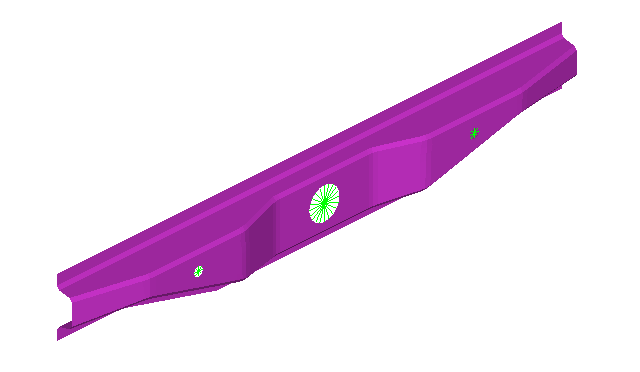
    The above pch file is generated from OptiStruct from a modal transient run.


    Figure 1.

Import the Model

  1. From the Home tools, Files tool group, click the Open Model tool.


    Figure 2.
  2. From the Load model and result dialog, browse and select HL-1100\Rear_Truss.h3d for the model file.
    The Load Result field is automatically populated. For this tutorial, the same file is used for both the model and the result.
  3. Click Apply.


    Figure 3.
Tip: Quickly import the model by dragging and dropping the .h3d file from a windows browser into the HyperLife modeling window.

Define the Fatigue Module

  1. From the Setup tools, click the SN tool.
    The SN tool should be the default fatigue module selected. If it is not, click the arrow next to the fatigue module icon to display a list of available options.


    Figure 4.
    The SN dialog opens.
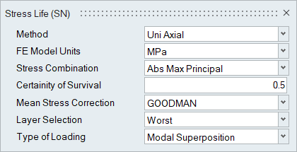
  2. Define the SN configuration parameters.
    1. Select Uni Axial as the method.
    2. Select MPa for the FE model units.
    3. Select Abs Max Principal for the stress combination
    4. Enter a value of 0.5 for the certainty of survival.
    5. Select GOODMAN for the mean stress connection.
    6. Select Worst for the layer selection.
    7. Select Modal Superposition for the type of loading.


    Figure 5.
  3. Exit the dialog.

Assign Materials

  1. From the Setup tools, click the Material tool.


    Figure 6.
    The Assign Material dialog opens.
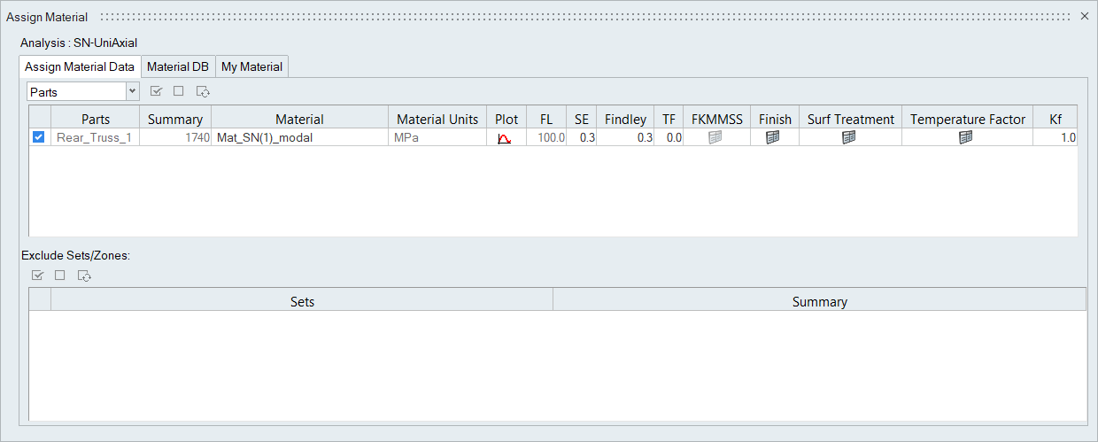
  2. Activate the checkbox next to the part Rear_Truss_1.
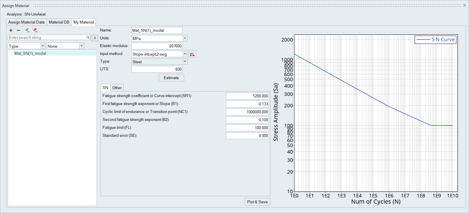
  3. Create a new material.
    1. Click the My Material tab.
    2. Click to create a new material.
    3. Name the material Mat_SN(1)_modal
    4. Set the Elastic modulus to 207000.
    5. Change the Input method to Slope-intcept,2-seg.
    6. In the SN tab, set the Fatigue strength coefficient or Curve intercept (SR1) to 1208.
    7. Set the Fatigue limit to 100.
    8. Set the Standard error to 0.3.
    9. Click the Other tab and ensure that the Yield strength is set to 250 and Poisson's Ratio is set to 0.333.
    10. Accept all other default settings then click Plot & Save.


      Figure 7.
  4. Right-click on Mat_SN(1)_modal and select Add to Assign Material List.
  5. Return to the Assign Material Data tab and select Mat_SN(1)_modal from the Material drop-down menu for Rear_Truss_1.
    The Material list is populated with the materials selected from Material Database and My Material.


    Figure 8.
  6. Exit the dialog.

Assign Load Histories

  1. From the Setup tools, click the Load Map tool.


    Figure 9.
    The Load Map dialog opens.
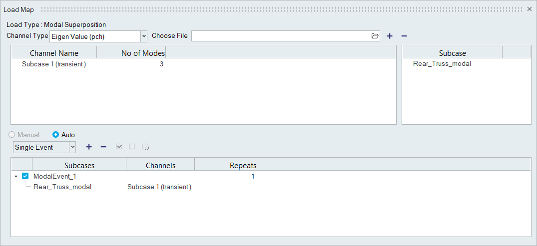
  2. From the Channel Type drop-down menu at the top of the dialog, select Eigen Value (pch).
  3. Click in the Choose File field and browse for Rear_Truss_modal.pch.
  4. Click to add the modal participation file.
  5. Select both the loaded pch file and the FE subcase Rear_Truss_modal.
  6. On the bottom half of the dialog, click .
    ModalEvent_1 is created with 1 repeat.
  7. Activate the ModalEvent_1 checkbox.


    Figure 10.
  8. Exit the dialog.

Evaluate and View Results

  1. From the Evaluate tool group, click the Run Analysis tool.


    Figure 11.
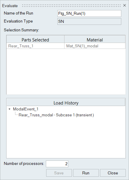
    The Evaluate dialog opens.


    Figure 12.
  2. Optional: Enter a name for the run.
  3. Click Run.
    Result files are saved to the home directory and the Run Status dialog opens.
  4. Once the run is complete, click View Current Results.
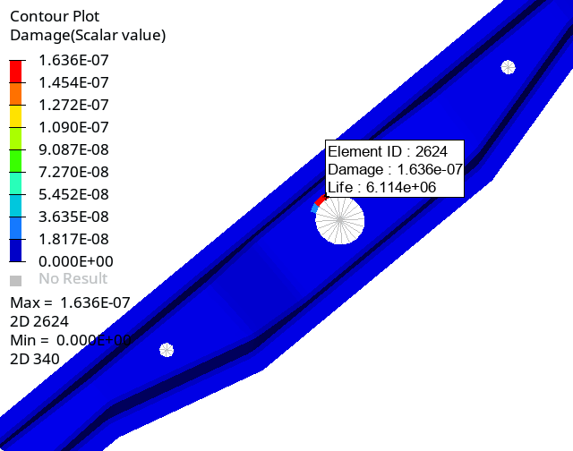
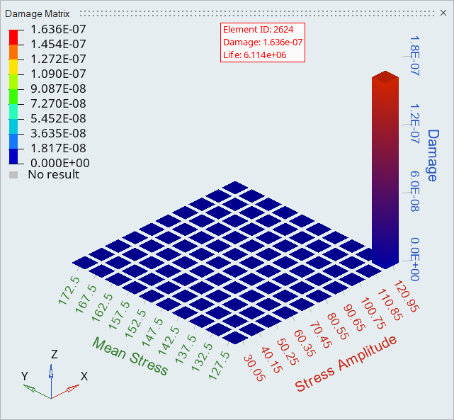
  5. Use the Results Explorer to visualize various types of results.


    Figure 13.


    Figure 14.