Guidelines for Optimization
Follow these guidelines when performing an optimization.
Always review the optimization log file
The optimization log file outputs information pertinent to the optimization process that was executed. Always review the log file to make sure that the optimization occurred without any difficulties. If the optimization has failed, the log file will tell you why the optimizer failed. This will give you a clue as to what the root cause of the issue is.
Sometimes, because the design limits are tight, the solution can get “stuck” at the boundary. In such a case, it is not unusual for the optimization to make very slow or no progress. The log file detects this situation and it will tell you this is the case. See the example below.
Results from Optimization
-------------------------
Initial Cost   = 11367.896
Final Cost     = 57.334
Cost reduction = 99.496

Individual Responses
--------------------
Weight = 1.00 Final cost of objective Coupler-DX  = 31.55
Weight = 1.00 Final cost of objective Coupler-DY  = 19.11
Weight = 1.00 Final cost of objective Coupler-PSI = 6.67


Final Design Table
------------------

DV                Lower Bound        Upper Bound        Initial Value      Optimized Value
------------------------------------------------------------------------------------------
XA                -5.0000e+01        +5.0000e+01        -4.5000e+01        -9.9618e+00
YA                -5.0000e+01        +5.0000e+01        +4.5000e+01        -1.1489e+01
XB                +2.0000e+01        +3.0000e+01        +2.5000e+01        +3.0000e+01  **** U
YB                +1.8000e+02        +1.9000e+02        +2.6000e+02        +1.8940e+02
XC                +2.4000e+02        +3.8000e+02        +3.0000e+02        +3.6508e+02
YC                +4.0000e+02        +6.2000e+02        +5.0000e+02        +6.0576e+02
XD                +1.8000e+02        +5.2000e+02        +5.1500e+02        +3.9105e+02
YD                -1.0000e+02        +2.0000e+01        -8.5000e+01        +1.6394e+01


**** You may consider expanding bounds for these DVs and re-run
MotionSolve appends **** U or **** U in the Final Design Table. The **** alerts you to the fact that the design is stuck at a boundary. The U tells you that the design is at the upper boundary. The L tells you that the design is at the upper boundary. In this example, if you want the optimization to find a better solution, you need to expand the upper design limit for XB.
Chose the right set of design variables for the problem
There are many ways to parameterize a design problem. Some parameterizations are more stable than others. Below is an example.
- One way to parameterize the profile is to create design variables for the (x ,y) coordinates of specific points on the profile. This is shown in the figure on the top.
- Another parameterization is to consider the radial length at a specific angular value as a design variable. You can choose the angular increments θ. This is shown in the figure on the bottom.
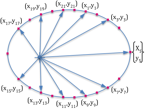
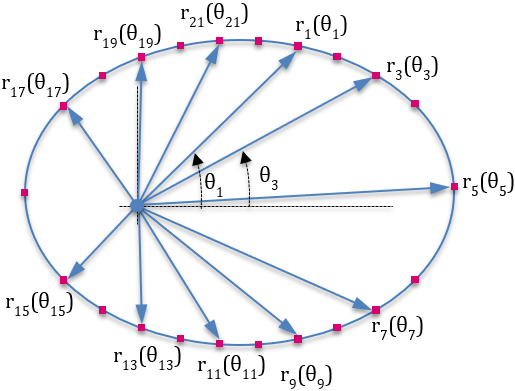
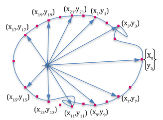
The parameterization with radial lengths (figure on bottom) is better for synthesizing the curve shape because it ensures that that the optimization cannot find a curve that does not have anomalies such as those shown below.
Make sure the design parameterization is correct
- One way to detect faulty parameterization is to generate models with different design parameters, perform simulations and examine the results. By examining the results closely, you may be able to identify the flaw in the parameterization.
- A second way to detect faulty parameterization is to look at the sensitivity of the responses to the design variables. This approach requires that you have some idea of what the sensitivities are. Some obvious mistakes can be identified with this approach. For instance, if the sensitivity of all responses to a certain design variable is always zero, it indicates that the particular design variable has no effect on the system performance. This could be due to an error in the parameterization.
Make sure the simulation is robust prior to optimization
A common cause for optimization failure is that the underlying simulation failed for some reason. Therefore, it is important to ensure that the underlying simulation is robust to changes in design before launching an (expensive) optimization run.
Manually change the initial design and run some simulations. Simulations should run without any warnings, static analyses should complete flawlessly, and time stepping for both dynamics and statics should occur without unexpected convergence failures. If this is not the case, examine and modify the model or the simulation settings such that the simulations are robust.
Specify realistic upper and lower bounds (bL, bU) for design variables
- Make sure that design variables that cannot be less than zero have a lower bound greater than zero. This is true for spring constants, damping coefficients and link lengths. These must always be greater than zero.
- Start with conservative values for lower and upper bounds, such as a restricted design space, so that the design variables are allowed only a little leeway to change. Iteratively, relax the design space so that the optimizer has room to find an optimum.
Use a crawl-walk-run approach to optimize your system
- Design variables
- Inequality constraints
- Equality constraints
- Cost functions
Introduce a few design variables at a time and successfully solve a design sub-problem before you attempt to solve a complex problem involving dozens of design variables.
Follow the same approach for the introduction of constraints. Introduce them a few at a time (one is ideal) and make sure the optimization continues to run and provides meaningful results before you introduce more constraints.
Sometimes, equality constraints may cause problems with the optimizer. If you find that this is the case, recast these as inequality constraints. Thus, if f(q, b) = 0 is an equality constraint, recast it as f(q, b) < 0 and f(q, b) > 0
When solving a multi-objective problem, make sure that the optimizer can find a solution when there is only one cost. Test each of the cost functions in this manner, before specifying all of them as the cost.
Look at intermediate results
The optimization process stores all the intermediate results. When an optimization fails, it is often quite instructive to review the intermediate results to see what the optimizer was doing. This may help you understand why the optimization failed.
If you forgot to specify a constraint on the design, you may see that the optimizer created a design that ideally, it should not have been allowed to.
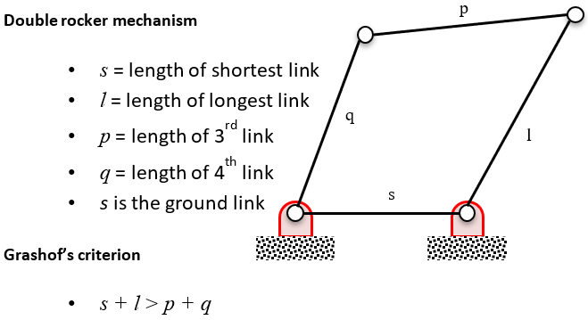
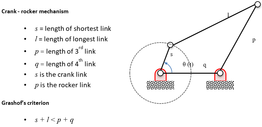
For mechanisms, enforce Grashof’s criterion where applicable
Use the debug feature built into the optimization module
Every Response can be optionally defined with its debug property set to True. When the debug property is true, the Response prints out its value whenever it is evaluated.
An alternative is to set the class variable, Response.debug = True. When this is done, all Responses print out their value whenever they are evaluated.
This will help you understand how the Responses are behaving during the optimization as the design changes.