Combine Modal Reduction

A domain decomposition method allowing the combination of nonlinear sub-domains with linear modal sub-domains has been proposed ¹. With this technique, the displacement field in the linear sub-domains is projected on a local basis of reduction modes calculated on the detailed geometry and the kinematic continuity relations are written at the interface in order to recombine the physical kinematic quantities of reduced sub-domains locally. The method yields promising save of computing time in industrial applications. However, the use of modal projection is limited to linear sub-domains. In the case of overall rigid-body motion with small local vibrations, the geometrical nonlinearity of sub-domains must be taken into account. Therefore, the projection cannot be used directly even thought the global displacements may still be described by a small number of unknowns; for example six variables to express motion of local frame plus a set of modal coordinates in this frame. This approach is used in the case of implicit framework. ² In the case of direct integration with an explicit scheme an efficient approach is presented. ³ One of the main problems is to determine the stability conditions for the explicit integration scheme when the classical rotation parameters as Euler angles or spin vectors are used. A new set of parameters, based on the so-called frame-mass concept is introduced to describe the global rigid body motion. The position and the orientation of the local frame are given by four points where the distances between the points are kept constant during the motion. In this way, only the displacement type DOF is dealt and the equations of motion are derived to satisfy perfectly the stability conditions. This approach, which was integrated in Radioss V5, will be presented briefly here.

A modal reduction basis is defined on one or more sub-domains of the decomposition. The definition of this basis is completely arbitrary. Any combination of eigen modes and static corrections can be used. All these modes are orthogonalized with respect to the finite element mass matrix in order for the projected mass matrix to be diagonal and suitable for an explicit solver.

Considering the case of a structure divided into two sub-domains, assume that modal reduction is used for linear Sub-domain 1. Thus, the displacement field of this sub-domain is projected onto the reduction vectors:(1)

U_{1} (t) = n \sum 1 α_{1}_{i} (t) Φ_{1}_{i} = Φ_{1} α_{1} (t)

$U_{1} (t) = \sum_{1}^{n} α_{1}_{i} (t) Φ_{1}_{i} = Φ_{1} α_{1} (t)$

with

$U_{1}$ vector of discretized displacements in Sub-domain 1,

$α_{1}$ vector of modal participations. This naturally yields:(2)

$\begin{array}{l} {\dot{U}}_{1} = Φ_{1} {\dot{α}}_{1} \\ {\ddot{U}}_{1} = Φ_{1} {\ddot{α}}_{1} \end{array}$

The number of modal unknowns $α_{1}$ chosen is much smaller than the original number of degrees of freedom of Sub-domain 1.

In order to obtain the new coupled system, the dynamic equilibrium of sub-domain 1 must be projected onto the reduction basis and the velocities involved in the kinematic relations must be expressed in terms of the modal coordinates. Thus, write the new matrix system for a single time scale as:(3)

$[\begin{matrix} \frac{Δ t}{2} {\hat{M}}_{1} & 0 & - \frac{Δ t}{2} {\hat{C}}_{1}^{T} \\ 0 & \frac{Δ t}{2} M_{2} & - \frac{Δ t}{2} C_{2}^{T} \\ - \frac{Δ t}{2} {\hat{C}}_{1} & - \frac{Δ t}{2} C_{2} & 0 \end{matrix}] [\begin{matrix} {\ddot{α}}_{1}^{n + 1} \\ {\ddot{U}}_{2}^{n + 1} \\ Λ \end{matrix}] = [\begin{matrix} \frac{Δ t}{2} {\hat{F}}_{1}^{n + 1} \\ \frac{Δ t}{2} F_{2}^{n + 1} \\ {\hat{C}}_{1} {}^{P}{\dot{α}}_{1}^{n + 1} + C_{2} {}^{P}{\dot{U}}_{2}^{n + 1} \end{matrix}]$

Where, (4)

$\begin{array}{l} {\hat{M}}_{1} = Φ_{1}^{T} M_{1} Φ_{1} \\ {\hat{F}}_{1} = Φ_{1}^{T} F_{e x t}_{1} - {\hat{K}}_{1} α_{1} \\ {\hat{K}}_{1} = Φ_{1}^{T} K_{1} Φ_{1} \\ {\hat{C}}_{1} = C_{1} Φ_{1} \end{array}$

The structure of this system is strictly identical to that which existed before reduction. Therefore, use exactly the same resolution process and apply the multi-time-step algorithm.

The time step for a reduced sub-domain is deduced from the highest eigen frequency of the projected system in order to preserve the stability of the explicit time integration. This time step is often larger than that given by the Courant condition with the finite element model before reduction.

Model Reduction with Finite Overall Rotation

Since large rotations are highly nonlinear ⁴, the displacement field in a sub-domain undergoing finite rotations cannot be expressed as a linear combination of constant modes. However, the rigid contribution to the displacement field creates no strain. In the case of small strains and linear behavior, the local vibrating system can still be projected onto a basis of local reduction modes. Then, take into account the rotation matrix from the initial global coordinate system to the local coordinate system and its time derivatives. A classical parameterization of this rotation, for example, Euler angles, would introduce nonlinear terms involving velocities. Since these quantities, in the central difference scheme, are implicit, this would require internal iterations in order to solve the equilibrium problem, a situation you clearly want to reduce the computation time due to the reduction.

Classically, the displacement field of a rotating and vibrating sub-domain is decomposed into a finite rigid-body contribution and a small-amplitude vibratory contribution measured in a local frame. The large rigid motion is represented using the so-called four-mass approach. ³

Four points

$(O, A, B, C)$ in space are arbitrarily chosen to represent the position of a local frame attached to the sub-domain. In order to simplify the local equations, choose these points so that they constitute an ortho-normal frame.

Note: The four points defining the local frame do not have to coincide with nodes of the mesh.

Displacement Field Decomposition

The global displacements of these four points are the unknowns describing the rigid motion of the sub-domain. These are classical displacement-type parameters. The relative distances between these points are kept constant during the dynamic calculation through external links. This enables us to express the total continuous displacement field of the sub-domain as:(5)

$u = X u_{A} + Y u_{B} + Z u_{C} + (1 - X - Y - Z) u_{O} + {Pu}_{L} = u_{E} + {Pu}_{L}$

Where,

$X, Y, Z$: Coordinates in the local frame $[O, A, B, C]$
$P$: Rotation matrix expressing the transformation from the local to the global coordinates: since $(\vec{O A}, \vec{O B}, \vec{O C})$ are unit vectors, $P = {[\vec{O A}; \vec{O B}; \vec{O C}]}^{}$ .

In order to express the dynamic equilibrium, Equation 4 must be derived with respect to time to yield velocities and accelerations.(6)

$\begin{array}{l} \dot{u} = X {\dot{u}}_{A} + Y {\dot{u}}_{B} + Z {\dot{u}}_{C} + (1 - X - Y - Z) {\dot{u}}_{O} + \dot{P} u_{L} + P {\dot{u}}_{L} \\ \ddot{u} = X {\ddot{u}}_{A} + Y {\ddot{u}}_{B} + Z {\ddot{u}}_{C} + (1 - X - Y - Z) {\ddot{u}}_{O} + \ddot{P} u_{L} + P {\ddot{u}}_{L} + 2 \dot{P} {\dot{u}}_{L} \end{array}$

The time derivatives of the rotation matrix are given by:(7)

$\begin{array}{l} \dot{P} = [{\dot{u}}_{A} - {\dot{u}}_{O}; {\dot{u}}_{B} - {\dot{u}}_{O}; {\dot{u}}_{C} - {\dot{u}}_{O}] \\ \ddot{P} = [{\ddot{u}}_{A} - {\ddot{u}}_{O}; {\ddot{u}}_{B} - {\ddot{u}}_{O}; {\ddot{u}}_{C} - {\ddot{u}}_{O}] \end{array}$

Thus, the fields in Equation 6 have the following expression:(8)

Where,

$u_{L}^{X}, u_{L}^{Y}, u_{L}^{Z}$ are the components of the local displacement in the local frame. The assumption of small perturbations in the local frame enables us to consider that the rigid and the deformed configurations are the same, that is, you can neglect

$u_{L}^{X}, u_{L}^{Y}, u_{L}^{Z}$ compared to the local coordinates,

$X, Y, Z$ . Thus, you get simplified expressions of the velocity and acceleration fields:(9)

$\begin{array}{l} \dot{u} = X {\dot{u}}_{A} + Y {\dot{u}}_{B} + Z {\dot{u}}_{C} + (1 - X - Y - Z) {\dot{u}}_{O} + \dot{P} u_{L} \\ \ddot{u} = X {\ddot{u}}_{A} + Y {\ddot{u}}_{B} + Z {\ddot{u}}_{C} + (1 - X - Y - Z) {\ddot{u}}_{O} + P {\ddot{u}}_{L} + 2 \dot{P} {\dot{u}}_{L} \end{array}$

To express the weak form of the dynamic equilibrium, you also need the variation

$δu$ of the displacement field:(10)

$δ u = X δ u_{A} + Y δ u_{B} + Z δ u_{C} + (1 - X - Y - Z) δ u_{O} + δ P u_{L} + P δ u_{L}$

Where, $δ P = [δ u_{A} - δ u_{O}; δ u_{B} - δ u_{O}; δ u_{C} - δ u_{O}]$

Again, the same assumption as above allows us to simplify this expression:(11)

Local Reduced Dynamic System

The local dynamic equilibrium of the sub-domain is given by:(12)

$ρ \ddot{u} - f_{int} (u) = 0$

The principle of virtual work yields a weak form of this equilibrium, taking into account, Dirichlet-type boundary conditions:(13)

$\int_{Ω} ρ δ u^{T} \ddot{u} d Ω - \int_{Ω} δ u^{T} f_{int} (u) d Ω = 0$

Where,

$\forall δ u$: Verifies the kinematic boundary conditions
$Ω$: Volume of the sub-domain

To introduce Equation 4 into this weak form of the equilibrium, you must express with the new parameterization the virtual works of both the internal and external forces and the virtual work, due to the rigid links among the points defining the local frame.

The internal forces can be calculated from the local part of the displacement, using Equation 5 and taking into account the rigid links, for example, the fact that displacement $u_{E}$ creates no strain.

(14)

$f_{int} (u) = P f_{int L} (u_{L}) = P d i v_{L} [σ_{L} (u_{L})]$

Where, index $L$ expresses that the coordinates and the spatial derivatives are taken in the local frame.

The virtual work of the internal forces is then:(15)

$δ W_{int} = \int_{Ω} δ u^{T} P d i v_{L} [σ_{L} (u_{L})] d Ω$

The integration by parts in the local frame introduces external surface forces

$f_{e x t}$ :(16)

Where,

$Γ$: The boundary of $Ω$
$n_{L}$: The normal to $Γ$ expressed in the local frame

To compute forces associated to the rigid links, first, new Lagrange multipliers are introduced to express the energy of a link:(17)

$W_{l i n k s} = \sum_{\begin{array}{l} (I, J) \in {(O, A, B, C)}^{2} \\ J > I \end{array}} Λ_{I J} D_{IJ} (u_{I}, u_{J})$

Where, $D_{I J} = ‖ (x_{I}^{0} + u_{I}) - (x_{J}^{0} + u_{J}) ‖ - ‖ x_{I}^{0} - x_{J}^{0} ‖$ and $x_{I}^{0}$ are the initial coordinates of point $I$ and the rigid link between points $I$ and $J$ is given by: $D_{I J} (u_{I}, u_{J}) = 0$ .

Then, the differentiation of this energy is used to obtain the virtual work to be introduced into the weak form of the equilibrium:(18)

$δ W_{l i n k s} = - \sum_{\begin{array}{l} (I, J) \in {(O, A, B, C)}^{2} \\ J > I \end{array}} δ Λ_{I J} D_{I J} (u_{I}, u_{j}) - \sum_{\begin{array}{l} I \in (O, A, B, C) \end{array}} δ u_{I} \sum_{\begin{array}{l} J \in (O, A, B, C) \\ J \neq I \end{array}} δ Λ_{I J} \frac{D_{I J} (u_{I}, u_{j})}{\partial u_{I}}$

(19)

$\forall δ u_{I} I \in (O, A, B, C)$

Note: The quantity

$\sum_{\begin{matrix} J \in (O, A, B, C) \\ J \neq I \end{matrix}} Λ_{I J} \frac{\partial D_{I J} (u_{I}, u_{J})}{\partial u_{I}} = F_{l i n k s}_{I J}$ can be viewed as the resisting force applied to point

$I$ to preserve the distances from this point to the other points of the local frame.

Weak Form of Equilibrium

Now, express the displacement field using Equation 5 and the local field projected on a Ritz basis:(20)

where $φ_{X}^{i} = X e_{i}$ , $φ_{Y}^{i} = Y e_{i}$ , $φ_{Z}^{i} = Z e_{i}$ , $φ_{1 - X - Y - Z}^{i} = (1 - X - Y - Z) e_{i}$ , $(e_{1}, e_{2}, e_{3})$ is a basis of the global frame, ${φ_{L}^{i}}^{}$ is a basis of local Ritz vectors obtained, for example, by finite element discretization or by modal analysis, $\hat{U}$ is the vector of the discrete unknowns:

$\hat{U} = [\begin{matrix} {[u_{A}^{i}]}_{} \\ {[u_{B}^{i}]}_{} \\ {[u_{C}^{i}]}_{} \\ {[u_{O}^{i}]}_{} \\ {[y^{i}]}_{} \end{matrix}] = [\begin{matrix} {\hat{U}}_{E} \\ {\hat{U}}_{L} \end{matrix}]$ , with ${\hat{U}}_{E} = [\begin{matrix} {[u_{A}^{i}]}_{} \\ {[u_{B}^{i}]}_{} \\ {[u_{C}^{i}]}_{} \\ {[u_{O}^{i}]}_{} \end{matrix}]$ and ${\hat{U}}_{L} = {[y^{i}]}^{}$ ,

$Φ_{P}$ is the projection basis: $Φ_{P} = {[{φ_{X}^{i}}, {φ_{Y}^{i}}, {φ_{Z}^{i}}, {φ_{1 - X - Y - Z}^{i}}, {{Pφ}_{L}^{i}}]}^{} = [Φ_{E}, {PΦ}_{L}]$ .

Equation 9 and Equation 11 yield:(21)

$\begin{array}{l} \dot{u} = Φ_{P} \dot{\hat{U}} \\ \ddot{u} = Φ_{P} \ddot{\hat{U}} + G (\dot{\hat{U}}) \\ δ u = Φ_{P} δ \hat{U} \end{array}$

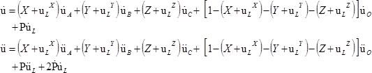
Where, $G (\dot{\hat{U}})$ is the gyroscopic contribution to the acceleration, given by:

$G (\dot{\hat{U}}) = 2 \dot{P} ([{\dot{u}}_{A}^{i}], [{\dot{u}}_{B}^{i}], [{\dot{u}}_{C}^{i}], [{\dot{u}}_{O}^{i}]) Φ_{L} {\dot{\hat{U}}}_{L}$

The final expression of the complete weak form of the dynamic equilibrium is obtained as:(22)

$\begin{array}{l} \int_{Ω} δ {\hat{U}}^{T} (Φ_{P}^{T}) Φ_{P} \ddot{\hat{U}} ρ d Ω + \int_{Ω} δ {\hat{U}}^{T} (Φ_{P}^{T}) G (\dot{\hat{U}}) ρ d Ω + \int_{Ω} σ_{L} (Φ_{L} {\hat{U}}_{L}) : ε_{L} (Ψ_{P} δ \hat{U}) d Ω \\ - δ Λ^{T} D ({\hat{U}}_{E}) - δ {\hat{U}}_{E}^{T} F_{l i n k s} (Λ, {\hat{U}}_{E}) = \int_{Γ} δ {\hat{U}}^{T} (Φ_{P}^{T}) f_{e x t} d S \end{array}$

Where,

$Φ_{L} = {ϕ_{L}^{i}}$

$ψ_{P} = [{P^{T} ϕ_{X}^{i}}, {P^{T} ϕ_{Y}^{i}}, {P^{T} ϕ_{Z}^{i}}, {P^{T} ϕ_{1 - X - Y - Z}^{i}}, {ϕ_{L}^{i}}] = [P^{T} Φ_{E}^{}, Φ_{L}^{}]$

$D$: Vector formed by the 6 relations preserving the relative distances of points $(O, A, B, C)$
$Λ$: Vector of the Lagrange multipliers corresponding to each rigid link
$F_{links}$: Vector of the link forces given by Equation 19

Equation 22 can be rewritten using classical matrix and vector operators obtained by finite element discretization:(23)

$δ {\hat{U}}^{T} M_{P} \ddot{\hat{U}} + δ {\hat{U}}^{T} F_{g y r} (\dot{\hat{U}}) + δ {\hat{U}}^{T} K_{L} {\hat{U}}_{L} - δ Λ^{T} D ({\hat{U}}_{E}) - δ {\hat{U}}_{E}^{T} F_{l i n k s} (Λ, {\hat{U}}_{E}) = δ {\hat{U}}^{T} F_{e x t}_{P}$

Where,

$M_{P} = {\bar{Φ}}_{P}^{T} {M \bar{Φ}}_{P}$ , with

$M$ being the classical mass matrix of sub-domain and

${\bar{Φ}}_{P}$ being the projection matrix consisting of vectors of

$Φ_{P}$ discretized on the nodes of the mesh:(24)

$F_{g y r} (\dot{\hat{U}}) = \int_{Ω} (Φ_{P}^{T}) G (\dot{\hat{U}}) ρ d Ω$

$K_{L} = {\bar{Ψ}}_{P}^{T} K {\bar{Φ}}_{L}$ , with $K$ being the sub-domain's local stiffness matrix and ${\bar{Ψ}}_{P}$ and ${\bar{Φ}}_{L}$ deduced (as was ${\bar{Φ}}_{L}$ ) from ${\bar{Ψ}}_{P}$ , ${\bar{Φ}}_{L}$ and the mesh, $F_{e x t}_{P} = {\bar{Φ}}_{P}^{T} F_{e x t}$ , with $F_{e x t}$ being the classical vector of the external forces assembled on the sub-domain.

Now, you are able to reduce the number of unknowns on the sub-domain drastically by choosing as the Ritz vectors, instead of classical finite element shape functions, an appropriate (and small) family of local reduction vectors. The modal vibration problem is purely local and guidelines found in the literature for the proper choice of the projection basis apply here.

Note: As far as inertia coupling with local vibration and overall large motion is concerned, two separate contributions must be considered. The first contribution appears in the projected mass matrix, which as now the following form:(25)

$M_{P} = [\begin{matrix} M_{E} & M_{_{C}}^{T} \\ M_{C} & M_{V} \end{matrix}]$

Where, $M_{E}$ is the constant mass matrix corresponding only to the global displacement field given by $X {\dot{u}}_{A} + Y {\dot{u}}_{B} + Z {\dot{u}}_{C} + (1 - X - Y - Z) {\dot{u}}_{O}$ , $M_{V}$ is the constant mass matrix corresponding to the local vibration given by $u_{L}$ , $M_{C}$ is a coupling matrix, variable with overall rotation, arising from the interaction between the local vibratory acceleration field expressed in the global frame $P {\ddot{u}}_{L}$ and the overall virtual displacement field $X δ u_{A} + Y δ u_{B} + Z δ u_{C} + (1 - X - Y - Z) δ u_{O}$ ; $M_{_{C}}^{T}$ naturally comes from the symmetric interaction between virtual local displacement field and the overall acceleration field.

The second contribution to the inertia coupling is the gyroscopic forces.

Note: In Radioss a special procedure is used to linearize the rigid links. ³

The rigid body motion component of the displacement increment is computed in unconditionally stable way by the use of Lagrange Multiplier to impose the rigid links. The deforming part is generated by the local vibration modes retained in the reduction basis. Therefore, you can conclude that the stability condition is the same as that given by the local vibrating system. The critical time step is constant throughout the calculation and can be derived from the highest eigen frequency of the local reduced stiffness matrix with respect to the local reduced mass matrix.

The highest eigen frequency

$f_{\max}$ is given by the system:(26)

$Φ_{L}^{T} K Φ_{L}^{} V = ω^{2} Φ_{L}^{T} M Φ_{L}^{} V$

Where, $Φ_{L} = {ϕ_{L}^{i}}^{}$ and $f = \frac{ω}{2 π}$ .

Having determined

$f_{\max}$ , the maximum time step which can be used on the reduced sub-domain while ensuring the stability of the time integration is:(27)

$Δ t_{\max} = \frac{1}{π f_{\max}}$

Faucher V. and Combescure A., “A time and space mortar method for coupling linear modal subdomains and nonlinear subdomains in explicit structural dynamics”, Computer Methods in Applied Mechanics and Engineering, Vol. 192, pp. 509-533, 2002.

Cardona A. and Géradin M., “A superelement formulation for mechanism analysis”, Computer Methods in Applied Mechanics and Engineering, Vol. 100, pp. 1-29, 1992.

Faucher V. and Combescure A., “Local modal reduction in explicit dynamics with domain decomposition. Part 1: extension to subdomains undergoing finite rigid rotations”, Int. Journal Num. Methods in Engineering, Vol. 60, pp. 2531-2560, 2004.

Argyris J.H., “An excursion into the large rotations”, Computer Methods in Applied Mechanics and Engineering, 32, 85-155, 1982.

Combine Modal Reduction

Linear Modal Reduction

Model Reduction with Finite Overall Rotation

Displacement Field Decomposition

Local Reduced Dynamic System

Weak Form of Equilibrium