RD-E: 1000 Bending

Pure bending test with different 3- and 4-nodes shell formulations.

The bending of a straight cantilever beam is studied. The example used is a famous bending test for shell elements. The analytical solution enables the comparison with the quality of the numerical results. Carefully watch the influence from the shell formulation. In addition, the results for the different time step scale factors are compared.

Options and Keywords Used

Q4 and T3 meshes
QEPH, Belytshcko & Tsay, BATOZ, and DKT shells
Mesh, hourglass, quasi-static analysis, and bending test
Imposed velocity (/IMPVEL)
Rigid bodies (/RBODY)

At one extremity of the beam, all DOF are blocked. A rotational velocity is imposed on the master node of the rigid body placed on the other side.

This velocity follows a linear function: Y=1

Input Files

The input files used in this example include:

BATOZ: <install_directory>/hwsolvers/demos/radioss/example/10_Bending/BATOZ/.../ROLLING*
QEPH: <install_directory>/hwsolvers/demos/radioss/example/10_Bending/QEPH/.../ROLLING*
BT (TYPE1): <install_directory>/hwsolvers/demos/radioss/example/10_Bending/BT/BT_type1/.../ROLLING*
BT (TYPE3): <install_directory>/hwsolvers/demos/radioss/example/10_Bending/BT/BT_type3/.../ROLLING*
BT (TYPE4): <install_directory>/hwsolvers/demos/radioss/example/10_Bending/BT/BT_type4/.../ROLLING*
DKT18: <install_directory>/hwsolvers/demos/radioss/example/10_Bending/DKT18/.../ROLLING*

Model Description

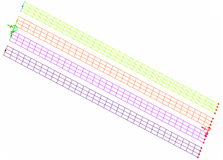
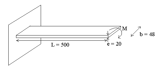
The purpose of this example is to study a pure bending problem. A cantilever beam with an end moment is studied. The moment variation is modeled by introducing a constant imposed velocity on the free end.

The following system is used: mm, ms, g, N, MPa

Several kinds of element formulation are used.

The material used follows a linear elastic law (/MAT/LAW1) with the following characteristics:

Material Properties
Initial density: 0.01 $[\frac{g}{m m^{3}}]$ $[\frac{g}{m m^{3}}]$
Reference density: .01 $[\frac{g}{m m^{3}}]$ $[\frac{g}{m m^{3}}]$
Young's modulus: 1000 $[MPa]$ $[MPa]$
Poisson ratio: 0

Model Method

The four models are integrated into one input file. The shell element formulations are:

Q4 mesh with the Belytshcko & Tsay formulation (I_shell =1, hourglass control TYPE1, TYPE2, and TYPE3)
Q4 mesh with the QEPH formulation (I_shell =24)
Q4 mesh with the QBAT formulation (I_shell =12)
T3 mesh with the DKT18 formulation (I_shell =12)

Results

Numerical Results and Analytical Solution Comparison

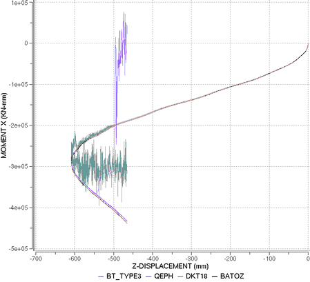
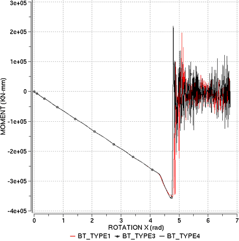
As shown in Figure 3, rotation around X and displacement with regard to Y of the free end are studied.

The analytical solution of the Timoshenko beam subjected to a tip moment reads:(1)

θ (z) = \frac{M z}{E I}

$θ (z) = \frac{M z}{E I}$

Which yields the end moment for a complete loop rotation

2 π

$2 π$ :(2)

M = \frac{2 π E I}{L} = \frac{2 π (1000) (\frac{48 * 20^{3}}{12})}{500} = 4.021 \times 10^{5} ​ KN-mm

$M = \frac{2 π E I}{L} = \frac{2 π (1000) (\frac{48 * 20^{3}}{12})}{500} = 4.021 \times 10^{5} KN-mm$

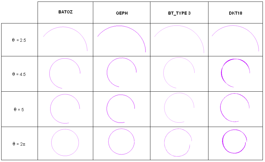
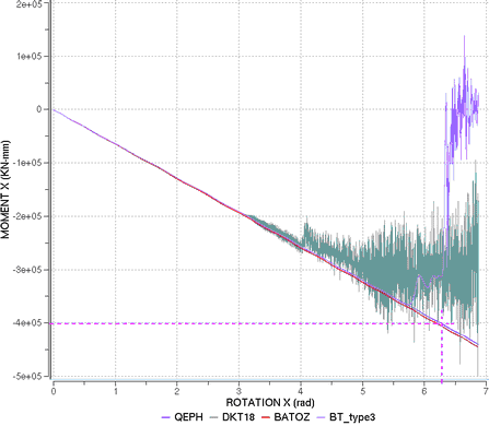
The following tables summarize the results obtained for the different formulations. From an analytical point of view, the beam deformed under pure bending must satisfy the conditions of the constant curvature which implies that for $θ$ $θ$ = $2 π$ $2 π$ , the beam should form a closed ring. However, depending on the finite element used, a small error can be observed, as shown in the following tables. This is mainly due to beam vibration during deformation as it is highly flexible. Good results are obtained by the QBAT, QEPH and DKT18 elements, respectively. This is mainly due to the good estimation of the curvature in the formulation of these elements. The BT family of under-integrated shell elements is less accurate. With the TYE3 hourglass formulation, the model remains stable until $θ$ $θ$ = 6rad. However, the moment-rotation curves do not correspond to the expected response.

To reduce the overall computation error, smaller explicit time steps are used by reducing the scale factor in /DT. The results reported in the end table show that a reduction in the time step enables to reduce the error accumulation, even though the divergence problems for BT elements cannot be avoided.

The following parameters are chosen for drawing curves and displaying animations:

	BATOZ	QEPH	BT	DKT
Scale factor	0.6	0.9	0.9	0.2
Imposed velocity rot.	0.005 rad/ms	0.005 rad/ms	0.005 rad/ms	0.005 rad/ms

The following curves show the evolution previously shown (rotation and nodal displacement by moment):

For

θ = 2 π \geq M_{A n a l y t i c a l} = - 4.021 \times 10^{5}

$θ = 2 π \geq M_{A n a l y t i c a l} = - 4.021 \times 10^{5}$

	BATOZ			QEPH		BT						DKT
	Sf=0.9	Sf =0.8	Sf =0.6	Sf =0.9	Sf =0.8	TYPE1		TYPE3		TYPE4		Sf =0.3	Sf =0.2	Sf =0.1
	Sf=0.9	Sf =0.8	Sf =0.6	Sf =0.9	Sf =0.8	Sf =0.9	Sf =0.1	Sf =0.9	Sf =0.1	Sf =0.9	Sf =0.1	Sf =0.3	Sf =0.2	Sf =0.1
CPU (normalized) # cycles	2.18 97600	2.43 109800	3.14 146400	1.23 95800	1.34 107800	42.64 59100	7.07 552600	2.62 182300	108.60 --	1.03 59100	7.17 552600	5.44 364100	8.21 621600	16.21 1243200
Error $θ$ $θ$ = 2 $π$ $π$ (%)	0%	0%	0%	0%	0%	55.3%	99%	0%	0%	55.9%	99.9%	3.4%	28.88%	3.7%
$θ$ $θ$ _{err =20%} (rad) degree	6.91 396°	6.89 395°	--	--	--	4.36 250°	4.53 260°	6.06 347°	5.98 343°	4.38 251°	4.51 258°	6.37 365°	--	--
Dz $θ$ $θ$ _{= 2 $π$ $π$} _(mm)	-500.5	-500.5	-500.5	-500.5	-500.5	-491.2	-525.8	-518.333	-506.0	-529.8	-433.8	-476.5	-496.5	-499.4
Mx $θ$ $θ$ _{= 2 $π$ $π$} _(x10⁺⁵_kN-mm)	-4.04	-4.05	-4.06	-4.01	-4.01	-0.21	-0.11	-3.13	-2.38	-0.07	-0.02	-3.09	-3.02	-3.08

Conclusion

A description summary of the different tests is:

QBAT element: This formulation gives a $2 π$ $2 π$ -revolution of the beam with no energy error. However, a 20% error is attained for $θ$ $θ$ = 384 degrees.; The decrease of the scale factor enables obtaining better results.
QEPH element: This formulation seems to be the best one to treat the problem. It enables a $2 π$ $2 π$ -revolution of the beam to be obtained. The error remains null until $θ$ $θ$ = 400 degrees.
BT formulation: This formulation does not provide satisfactory results and is not adapted to this simulation, whatever the anti-hourglass formulation. This is mainly due to using a flat plate formulation and the fact that the element is under-integrated. The TYPE3 hourglass formulation seems to be better than others.
DKT formulation: The bending is simulated correctly. However, the element is costly and the CPU time is much longer.