Compose-4020: Solving Differential Algebraic Equations
When a system of equations contains both algebraic and ordinary differential equations, it is a differential algebraic equation. The solution method is different than with ordinary differential equations. The differences are in how the user functions are defined and the need for initial conditions for the derivatives of the state variables as well.
This tutorial will solve the series RLC circuit, subject to a constant voltage by formulating it as a differential algebraic equation.
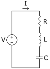
- VR = node voltage between the resistor and inductor
- VL = node voltage between the inductor and capacitor
- V = the voltage source
- I = the current in the circuit
- R = the resistor value
- C = the capacitor value
- L = the inductor value
A system of equations representing the circuit are shown below:
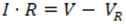

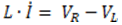
The state variables of the system are I, VR and VL. You will solve for their time-series values. Notice that the first equation is purely algebraic, meaning that it does not involve derivatives. This is what distinguishes the system from an ODE system.
Rewriting the Equations
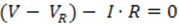
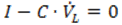
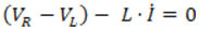
Unlike ordinary differential equations, differential algebraic systems must be rearranged in terms of residuals:
Implementing the Equations
-
From the File menu, select Open and locate the file
ode15iDemo.oml in
<installation_dir>/tutorials/ folder.
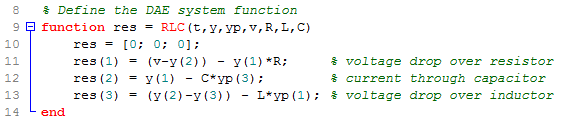
The system function looks like this, using y in the code for the vector [i, VR, VL].
 Define the circuit variables.
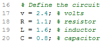
To solve the system, perform the following steps.
- Pass the circuit variables to the DAE system function using a handle.
- Define the times at which to solve the system.
- Define the initial values of [i, VR, VL] in
y. - Define the initial values of the [i, VR, VL]
derivatives in
yp. - Set tolerances. The defaults are explicitly specified below for illustration.
- Call
ode15iwith the inputs.
The code looks like this: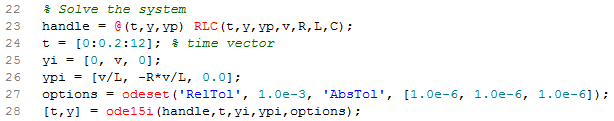
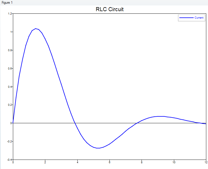
The time vector is reproduced as the first output argument. It is identical to the input for this case. The second output argument, v, contains the values of i, VR, VL by column at each time in vector t.
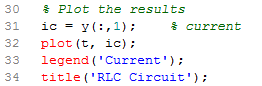
The following code extracts and plots the results.